

For more information click here for the Costing Climate Change to Public Infrastructure portal.
Glossary of Terms
List of Abbreviations
Term Definition
- CIPI
- Costing Climate Change Impacts to Public Infrastructure (project)
- CRV
- Current Replacement Value
- IDF
- Intensity-Duration-Frequency (Curve)
- IPCC
- Intergovernmental Panel on Climate Change
- O&M
- Operation and Maintenance
- RCP
- Representative Concentration Pathway
- SME
- Subject-Matter Expert
- USL
- Useful Service Life
- WSP
- WSP Global Inc.
Definitions
Current Replacement Value: The current cost of rebuilding an infrastructure asset with the equivalent capacity, functionality and performance.
Operations and Maintenance (O&M): The routine activities performed on an asset that maximize service life and minimize service disruptions.
Rehabilitation: Repairing part or most of an asset to extend its service life, without adding to its capacity, functionality or performance.
Renewal: Replacement of an existing asset, resulting in a new or as-new asset with an equivalent capacity, functionality and performance as the original asset. Renewal is different from rehabilitation, as renewal rebuilds the entire asset.
State of Good Repair: A performance standard which helps to maximize the benefits of public infrastructure in a cost-effective manner over time, and ensures that infrastructure operates in a condition that is considered acceptable from an engineering perspective.
Stable Climate: A stable climate scenario assumes that climate indicators for extreme rainfall, extreme heat and freeze-thaw cycles remain unchanged from their 1975-2005 average levels over the projection to 2100.
Rest of the Century: Refers to the 79 years from 2022 to 2100.
Baseline Cost: The operations and maintenance, rehabilitation, and renewal expense that would have been required to maintain public transportation infrastructure in a state of good repair in a stable climate.
Acute Hazard: Severeclimate hazards that occur rarely (such as the 100-year storm event).
Chronic Hazard: Climate hazards that occur often.
Retrofit: An adaptation made during the asset’s service life.
Adaptation: Adaptation is modelled as an alteration of an asset’s physical components to prevent more rapid deterioration and increased O&M expenses caused by changes in extreme rainfall, extreme heat and/or freeze-thaw cycles. Adaptation can be done through retrofit while an asset is still in service or can be done at the time of renewal.
No Adaptation Strategy / Damage Costs: An asset management strategy where public infrastructure assets are not adapted to changing climate hazards.
Reactive Adaptation Strategy: An asset management strategy where publicinfrastructure assets are only adapted at the time of renewal to withstand changing climate conditions.
Proactive Adaptation Strategy: An asset management strategywhere public infrastructure assets are adapted at the first available opportunity to withstand changing climate conditions. This occurs either during an asset’s next major rehabilitation through a retrofit or at renewal, whichever comes first.
1 | Introduction and context
In June 2019, a Member of Provincial Parliament asked the FAO to analyze the costs that climate change impacts could impose on Ontario’s provincial and municipal infrastructure, and how those costs could impact the long-term budget outlook of the province. In response to this request, the FAO launched its Costing Climate Change Impacts to Public Infrastructure project (CIPI).
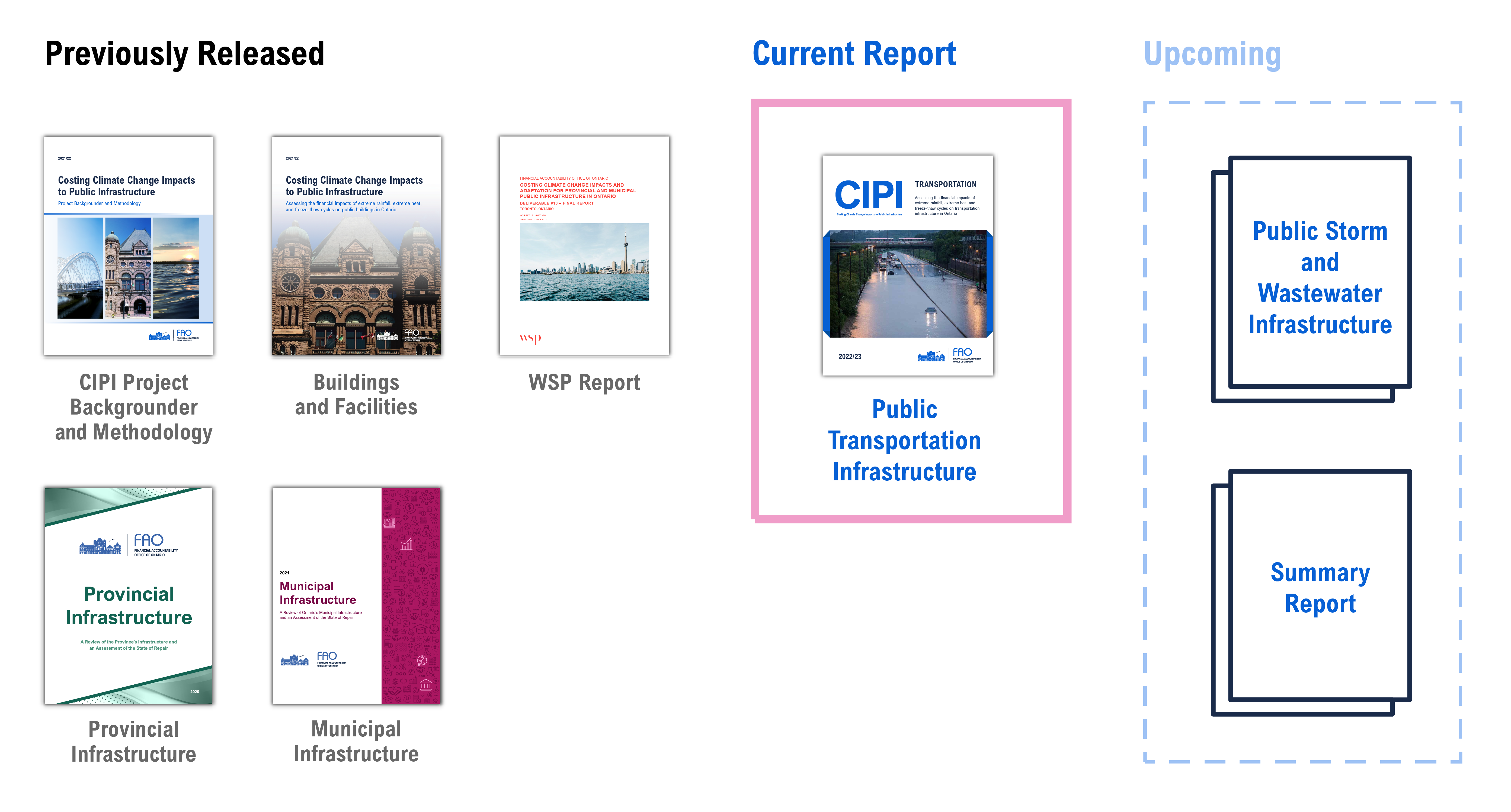
In the first two phases of the project, the FAO assessed the composition and state of repair of provincial[1] and municipal[2] infrastructure, with findings released in November 2020 and in August 2021. In fall 2021, the FAO released three reports: a project backgrounder[3] that describes the overall context and methodology of the CIPI project, a report prepared by WSP Global[4] that describes the detailed engineering impact of climate hazards on public infrastructure, and a report detailing how changes in extreme rainfall, extreme heat and freeze-thaw cycles will impact the long-term costs of maintaining Ontario’s public buildings and facilities in a state of good repair.[5]
This report examines how changes in extreme rainfall, extreme heat and freeze-thaw cycles will impact the long-term costs of maintaining public transportation infrastructure in a state of good repair.
2 | Summary
Ontario’s provincial and municipal governments manage a large portfolio of transportation infrastructure
These transportation assets, valued at $330 billion, include roads, bridges, large structural culverts and rail tracks. Ontario’s 444 municipalities own 82 per cent of this transportation infrastructure (or $269 billion), while the remaining 18 per cent ($61 billion) is owned by the Province (all costs are in 2020 real dollars).
The cost to maintain the existing portfolio in a state of good repair is substantial, even in a stable climate
If the climate was stable, it would cost $12.9 billion per year to bring these assets into a state of good repair and maintain them. Over the rest of the century, these costs would accumulate to approximately $1 trillion by 2100.
Changes in extreme rainfall, extreme heat and freeze-thaw cycles are already increasing the costs of maintaining Ontario’s public transportation infrastructure
In the absence of adaptation, these climate hazards are expected to increase the costs of maintaining Ontario’s transportation infrastructure by approximately $1.5 billion per year in this decade, above what would have occurred in a stable climate. By 2030, these climate-related costs would accumulate to $13.3 billion for provincial and municipal governments.
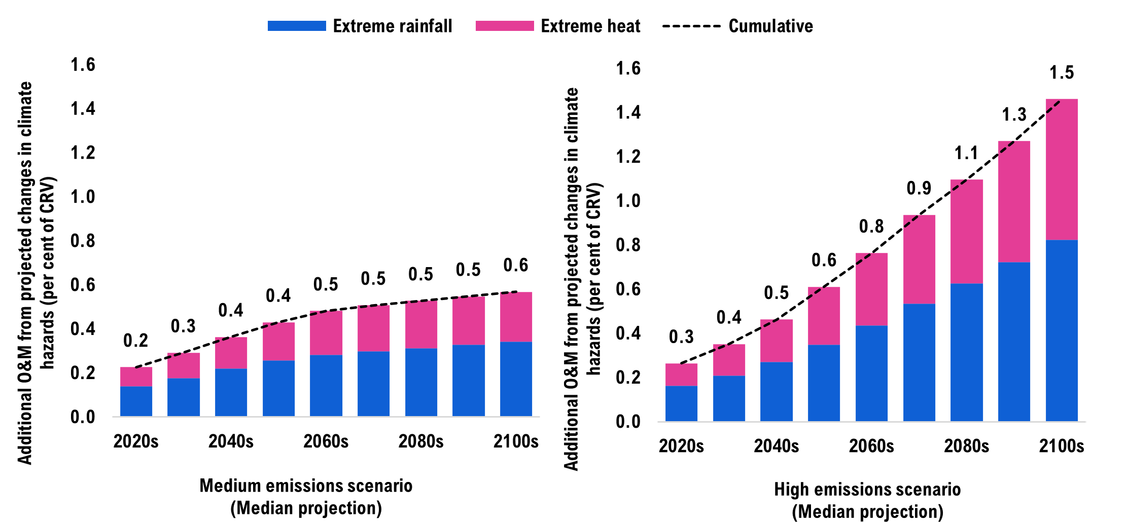
In the absence of adaptation, climate hazards will continue to increase the costs of maintaining Ontario’s public transportation infrastructure throughout the century
In a medium emissions scenario, where global emissions peak by mid-century, these climate hazards would increase infrastructure costs by an average of $2.2 billion per year, totalling $171 billion in additional costs by 2100. This is a 17 per cent increase in costs relative to a stable climate scenario. In the high emissions scenario, where global emissions continue rising throughout the century, transportation infrastructure costs would instead increase by $4.1 billion per year on average, totalling $322 billion by 2100. This is a 32 per cent increase in costs relative to a stable climate scenario.
Adapting public transportation infrastructure to withstand these climate hazards will cost less than not adapting over the long term
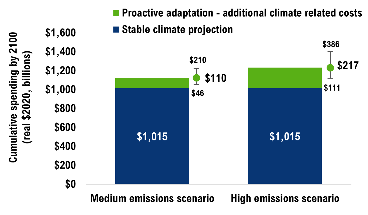
Depending on the emissions scenario, adapting public transportation infrastructure will add between $110 billion to $229 billion to infrastructure costs relative to a stable climate scenario by 2100. This represents a cost increase between 11 and 23 per cent. While significant, these additional climate-related costs are lower than those incurred in the absence of adaptation.
Costing climate impacts to public infrastructure over the long term is subject to significant uncertainty
The extent of global climate change will have a direct impact on Ontario’s public infrastructure costs. Climate-related costs will depend on the future path of global emissions, the vulnerability of infrastructure to changing climate hazards, and the pace of adaptation. The FAO’s study presents median cost projections as well as a range of possible cost outcomes in each scenario that account for this uncertainty.
This study focused on three climate hazards but excluded others, such as wildfires and ice storms. Costs to governments were estimated, but the broader economic costs to households or businesses from damaged transportation infrastructure were not included. These impacts were beyond the scope of this report but are likely material. These subjects would benefit from further research.
Figure 2-1 Adapting Ontario’s public transportation infrastructure will cost Provincial and municipal governments less than not adapting in a changing climate

Note: The costs in this chart are based on the median (or 50th percentile) projection under each emissions scenario and are in addition to the baseline costs over the same period. For presentation purposes, the uncertainty bands are not shown in this figure.
Source: FAO.
3 | The long-term costs of maintaining public transportation infrastructure
This chapter presents the scope of public transportation infrastructure considered in this report, discusses the costs necessary to maintain these assets in a state of good repair, and estimates the long-term infrastructure costs required to maintain infrastructure to 2100 under a stable climate. The purpose of this chapter is to establish a baseline projection of infrastructure costs. In later chapters, this baseline is compared to projections that account for changes in certain climate hazards.
There is a large portfolio of public transportation infrastructure in Ontario
This report focuses on transportation infrastructure owned and controlled by provincial and municipal governments. The FAO estimates that the current replacement value[6] (CRV) of these assets is at least $330 billion in 2022.[7] The public transportation assets included in the scope of this report are roads, bridges, large structural culverts as well as transit engineering assets:[8]
- Roads include arterial roads, collector roads, highways, lanes and alleys, local roads, rural highways, and sidewalks. In this report, road CRV represents the cost of road reconstruction.[9]
- Bridges include those located on arterial roads, collector roads, and highways, as well as local bridges and footbridges. Bridge CRV represents the cost of replacing a bridge with one of equal functionality.
- Large structural culverts include those greater than three metres in diameter. Culvert CRV represents the cost of replacing a culvert with one of equal functionality.
- Transit engineering assets include rail (tracks). Transit CRV represents the cost of replacing existing rail tracks.
Ontario’s municipal governments own $269 billion of the transportation infrastructure assets in scope (82 per cent), while the provincial government owns $61 billion (18 per cent).[10]
Figure 3-1 Ontario’s public transportation infrastructure covered in this report has a current replacement value of $330 billion
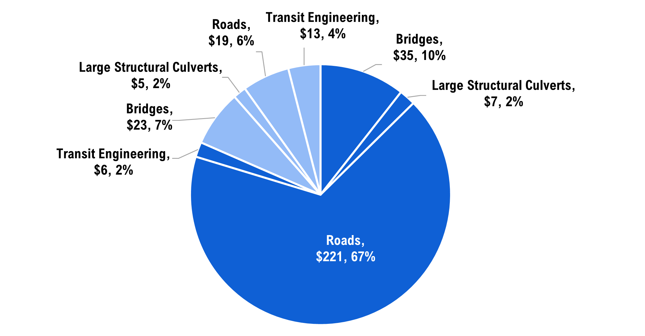
Note: CRV estimates are in real 2020 billion dollars. Percentage values refer to a sector’s share of total CRV.
Source: FAO.
Maintaining a large portfolio of public transportation infrastructure requires constant spending
Keeping assets in a state of good repair helps to maximize the benefits of public infrastructure in the most cost-effective manner over time. To be maintained in a state of good repair, assets require annual operations and maintenance (O&M) spending, as well as intermittent capital spending either to rehabilitate[11] an asset or renew it at the end of its service life.[12]
The costs to maintain public transportation infrastructure in a state of good repair reflect both the value of assets owned, as well as the condition, age and performance standards of each individual asset under management. For example, assets in poorer condition require more capital spending to bring them into a state of good repair. Likewise, older assets must be renewed sooner than newer assets.
To project the costs of maintaining public transportation infrastructure in a state of good repair, the FAO gathered and estimated asset-specific information on age, condition and current replacement value, as well as the general performance standards used to evaluate if an asset is in a state of good repair. Using an infrastructure deterioration model based on modelling techniques developed by the Ontario Ministry of Infrastructure,[13] the FAO projected the capital and operating expenses necessary to maintain the current portfolio[14] of public transportation infrastructure in a state of good repair to 2100, in the absence of climate considerations.[15]
These long-term O&M, rehabilitation, and renewal spending estimates form the baseline projection against which the climate change costing scenarios will be compared. The baseline projection represents the infrastructure costs that would have been required to maintain public transportation infrastructure in a stable climate.[16] This allows the FAO to identify the additional climate-related infrastructure costs that are associated with changing climate hazards in later chapters.
Given the long useful service life of public transportation infrastructure, costs are projected to 2100. The results in this report are presented as average annual costs, as well as cumulative total costs over the century. Average annual costs are also presented over three time periods.
- The short term (2022-2030) shows how changing climate hazards are already impacting public infrastructure costs in the current decade.
- The mid-century (2031-2070) captures the period in which projections for the relevant climate variables begin to diverge in the three global emissions scenarios examined in this report (see Figure 4-3).
- The late century (2071-2100) captures the period where projections for the relevant climate variables diverge significantly in the three global emissions scenarios examined in this report.
$12.9 billion per year needed to maintain the current portfolio of public transportation infrastructure in a stable climate
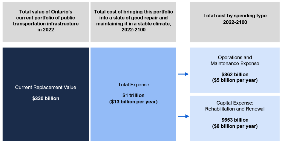
The FAO projects that bringing Ontario’s existing suite of public transportation infrastructure assets into a state of good repair and maintaining them until 2100 would have cost an average of $12.9 billion per year in a stable climate, which would accumulate to approximately $1 trillion by the end of the century. This cumulative baseline cost includes $362 billion ($4.6 billion per year) in O&M expense and $653 billion ($8.3 billion per year) in rehabilitation and renewal expense to 2100.
Figure 3-2 The costs of maintaining Ontario’s public transportation infrastructure in a state of good repair to 2100 in a stable climate (real 2020 dollars)
Source: FAO.
Accessible version
The current replacement value (CRV) of Ontario’s current portfolio of public transportation infrastructure in 2022 is $330 billion. In a stable climate, the cumulative cost of bringing and maintaining Ontario’s existing suite of public transportation infrastructure into a state of good repair until 2100 would be $1 trillion, or an average of $12.9 billion per year. This baseline cost includes $362 billion ($4.6 billion per year) in cumulative operations and maintenance (O&M) expense and $653 billion ($8.3 billion per year) in rehabilitation and renewal expense to 2100.
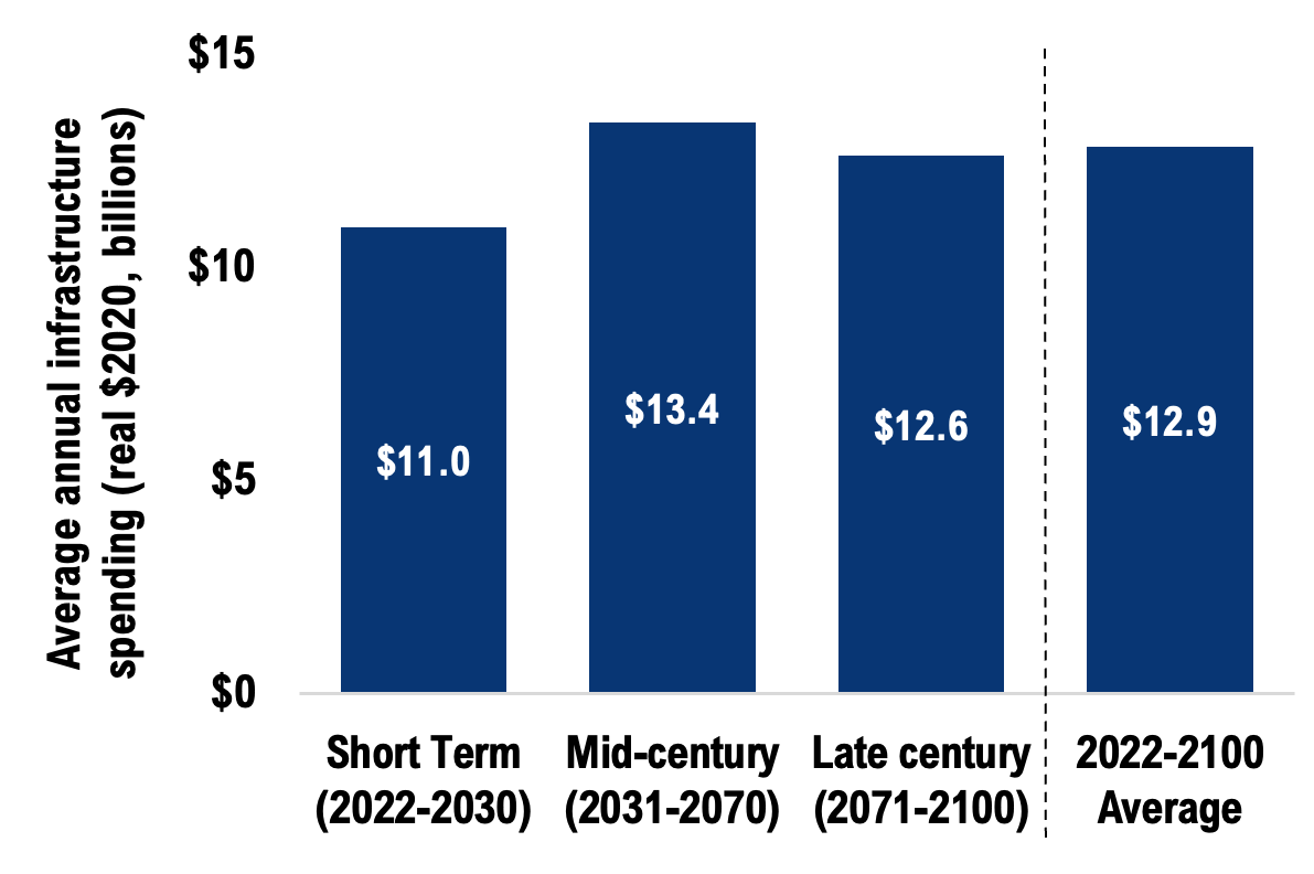
Figure 3-3 Maintaining Ontario’s public transportation infrastructure in a stable climate would have cost $12.9 billion per year
Source: FAO.
In the short term, provincial and municipal governments would need to spend approximately $11 billion per year to bring this portfolio of public transportation infrastructure into a state of good repair and maintain it. These average annual costs rise to $13.4 billion in the mid-century period, when a significant share of Ontario’s public transportation infrastructure begins to be replaced. By late century, it would take $12.6 billion per year to maintain this portfolio of public transportation infrastructure in a stable climate.
All infrastructure cost projections presented in this report assume that the funding necessary to bring and maintain the current portfolio of transportation infrastructure into a state of good repair is made available and spent in a timely manner. In practice, infrastructure repair backlogs exist and maintaining assets in a state of good repair is only one aspect of asset management. The baseline cost projection does not include any spending associated with assets either currently under construction, planned for future construction or necessary to meet future infrastructure demand.[17]
4 | The cost of key climate hazards to transportation infrastructure
Climate change is associated with many hazards to public infrastructure, which can take the form of extreme weather events or long-term chronic impacts. Ontario has been subject to costly floods and ice storms and is also prone to droughts, intense rainfall, wildfires, windstorms, heatwaves, and permafrost melt.[18] This project focuses on only three climate hazards – extreme rainfall, extreme heat and freeze-thaw cycles – as they were determined to have broad and financially material impacts to public infrastructure and can be projected with a reasonable degree of scientific confidence.[19]
This chapter summarizes how projected changes in these climate hazards would impact Ontario’s public transportation infrastructure in the absence of adaptation measures. It then presents the FAO’s estimates of the additional long-term costs these climate hazards would impose on Ontario’s portfolio of public transportation infrastructure in medium and high emissions scenarios.
Changing extreme rainfall, extreme heat and freeze-thaw cycles will impact transportation infrastructure
To ensure safety and reliability, infrastructure is designed, built and maintained to withstand a specific range of climate conditions typically based on historic climatic loads.[20] However, extreme rainfall and extreme heat are projected to increase in the future, while freeze-thaw cycles are projected to decrease.[21]
Changing climate hazards will impact transportation infrastructure assets in different ways. Of all the possible hazard–asset type interactions, this report examines six impacts: extreme rainfall and extreme heat on roads, extreme rainfall and freeze-thaw cycles on bridges, extreme rainfall on large structural culverts, and extreme heat on transit engineering (Figure 4-1). The following section provides an overview of how these climate hazards will impact the different asset types.[22]
Figure 4-1 Scope of interactions between selected climate hazards and public transportation asset types
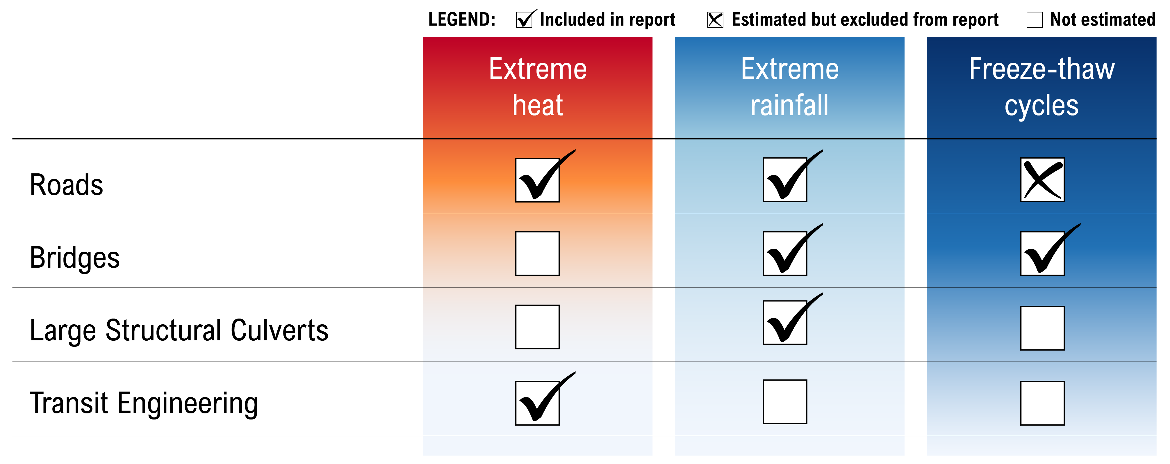
Source: WSP and FAO.
Roads
Extreme rainfall will impact road infrastructure most significantly in acute events (i.e., 100-year storm events[23]) as roads are typically considered resilient to less-intense rainfall events. Washouts and flooding during severe rainfall events can overwhelm drainage features and damage pavement. Extreme rainfall can also cause water to penetrate the base and sub-base materials, leading to increased deterioration and cracking.
Extreme heat in the form of ambient temperatures over 30°C creates conditions where heat dissipates less efficiently, softening the asphalt pavement. This increases the road’s vulnerability to rutting and cracking, which can lead to increased water infiltration, weakening the base/sub-base and causing surface issues such as potholes.
Freeze-thaw cycles (FTCs) are fluctuations between freezing and non-freezing temperatures that cause water to freeze (and expand) or melt (and contract). In contrast to vertical infrastructure (e.g., buildings) where less water accumulates due to gravity runoff, horizontal infrastructure like roads have the potential to accumulate water that penetrates sub-layers. The melting and re-freezing of accumulated water can then damage road surfaces. While the FAO conducted a preliminary analysis of this impact, there was low confidence in the costing results due to the lack of research on the combined impacts of moisture and frost conditions on roads. As such, the costing results for freeze-thaw cycles on roads were excluded from this report.
Bridges
Extreme rainfall will impact bridges as acute events (i.e., 100-year storm events) through runoff and flooding. These events will erode embankments and approaches, as well as scour and erode both bridge substructures and shallow bridge foundations. Deep bridge foundations will be negligibly impacted.
Freeze-thaw cycles contribute to the weathering of bridge decks and barriers, causing concrete cracking. However, the projected decline in the number of annual freeze-thaw cycles will increase the service life of vertical concrete. FTCs are not expected to significantly impact other bridge components, including the superstructure, substructure, and the layer below the asphalt pavement.[24]
Large Structural Culverts
Extreme rainfall will impact large structural culverts as acute events (i.e., 100-year storm events) through increased erosion. Channel protection will also be vulnerable to washout and scour damages.
Transit Engineering
Extreme heat in the form of chronically high ambient temperatures over 30°C can cause stress on steel rail tracks and other alignment components such as rail brace, tie plates and insulated joints. Higher temperatures also increase friction between train wheels and tracks, potentially resulting in track buckling. Just a few hours of above-average heat are enough to cause problems, with buckling probability increasing rapidly once temperatures exceed around 35°C.[25]
Figure 4-2 Examples of climate hazard impacts to key components of public transportation infrastructure
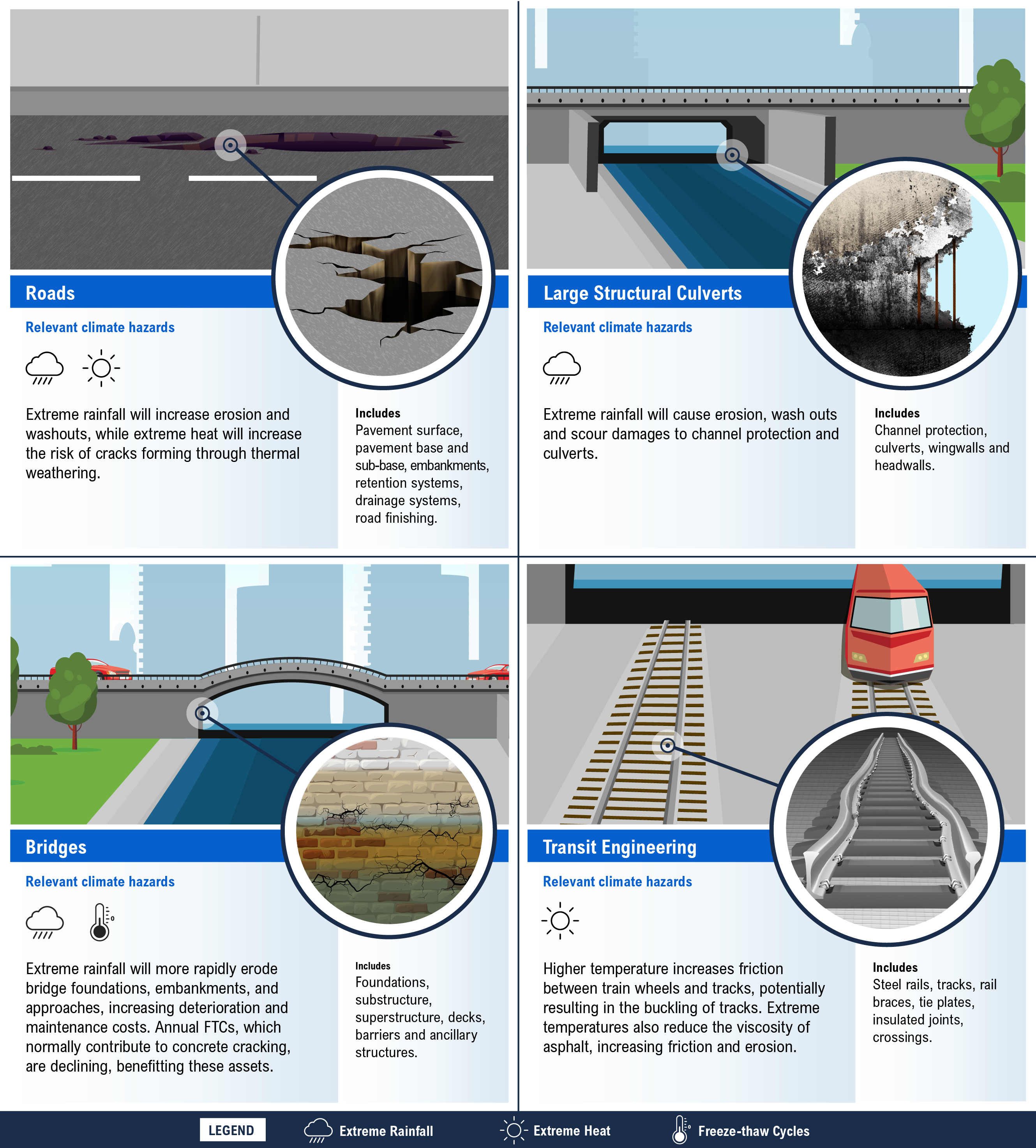
Note: For more examples of how these climate hazards impact transportation infrastructure, see WSP 2021.
Source: WSP.
Most climate hazards to public transportation infrastructure will increase
The impacts of changing climate hazards on Ontario’s public transportation infrastructure will depend on the path of global greenhouse gas emissions and the extent of global mean temperature increases. The FAO costed climate impacts to public transportation infrastructure for three global emissions scenarios:
- A low emissions scenario that assumes a major and immediate turnaround in global climate policies. Emissions are projected to peak in the early 2020s and decline to zero by the 2080s. By the end of the century, net emissions are negative. In this scenario, global mean temperatures are projected to increase by 1.6°C (0.8 to 2.4°C) by 2100 compared to the pre-industrial average (1850-1900).[26] The key results for this scenario are presented in Appendix F.
- A medium emissions scenario, where global emissions peak in the 2040s, then decline rapidly over the following four decades before stabilizing at the end of the century. In this scenario, the global mean temperature is projected to increase by 2.3°C (1.7 to 3.2°C) by 2100 relative to 1850-1900.
- A high emissions scenario that assumes global emissions continue to grow for most of the century.[27] Global mean temperatures are projected to increase by 4.2°C (3.2 to 5.4°C) relative to 1850-1900. Cumulative emissions from 2005 to 2020 most closely match the high emissions scenario.[28]
Uncertainty in climate change projections
The FAO partnered with the Canadian Centre for Climate Services at Environment and Climate Change Canada to acquire projections of key climate indicators for Ontario. To account for uncertainty in climate projections and in line with common practice in climate science, the median (50th percentile) projections of climate variables are presented, followed by ranges in parentheses. For Ontario climate indicators, the ranges indicate the 10th and 90th percentile projections from the ensemble of 24 climate models used by the Canadian Centre for Climate Services.
Figure 4-3 presents a brief description of the projected changes in the climate indicators used to represent these hazards. Appendix B contains a full description of all relevant climate variables to public transportation infrastructure, and their trends in all scenarios.
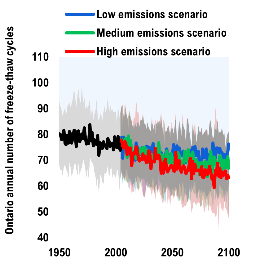
Figure 4-3 Changing climate hazards in Ontario
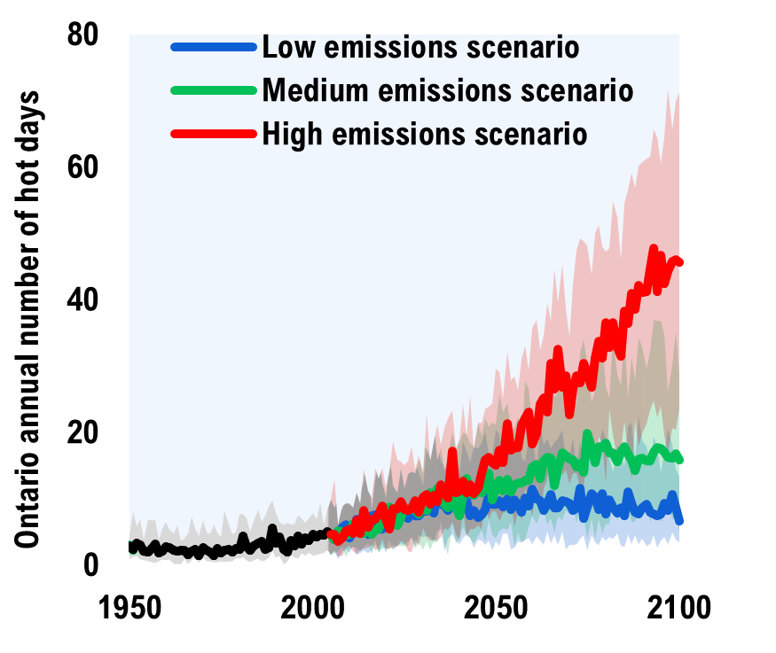
- Projected changes in Ontario’s annual number of hot days (number of days with daily maximum temperature above 30°C) differ significantly in the low and high emissions scenarios. Over the 1976-2005 period, there were on average 4 hot days every year. Compared to this baseline, Ontario’s annual number of hot days is projected to increase by 5 days (2 to 10 days) in the low emissions scenario and by 34 days (17 to 46 days) in the high emissions scenario by the 2071-2100 period.
- There is high confidence in the projected trends and ranges of temperature variables based on strong scientific evidence in the causes of observed changes.[29]
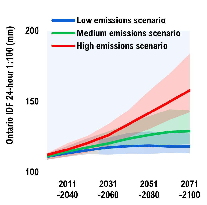
- Compared to the 1976-2005 baseline, the intensity of a 24-hour 1-in-100-year rainfall event in Ontario is projected to increase by 15 per cent (10 to 23 per cent) in the low emissions scenario and by 53 per cent (38 to 78 per cent) in the high emissions scenario by the 2071-2100 period.
- Over the 1976-2005 period, the average 1-in-100-year 24-hour rainfall in Ontario was 103 mm. By the 2071-2100 period, there is projected to be on average 118 mm (113 to 127 mm) of rain in the low emissions scenario and 158 mm (142 to 185 mm) of rain in the high emissions scenario.
- Confidence in the projected trends and ranges of aggregate precipitation variables is somewhat lower (medium) than for temperature variables as there is less confidence in how well climate models represent the climate processes involved.
- Annual FTCs are the number of days in a year when the temperature crosses 0°C. Over the coming decades, the winter season will shorten due to rising temperatures. Ontario’s annual FTCs are projected to decline by 5 per cent (0 to 15 per cent) in the low emissions scenario and by 15 per cent (0 to 25 per cent) in the high emissions scenario by the 2071-2100 period.
- Over the 1976-2005 period, there were on average 77 freeze-thaw cycles every year. Compared to this baseline, Ontario’s annual number of FTCs is projected to decrease by 4 cycles (-12 to 0 cycles) in the low emissions scenario and by 12 cycles (-19 to 0 cycles) in the high emissions scenario by the 2071-2100 period.
- There is high confidence in the projections of annual FTCs based on the amount of evidence for projected trends and ranges of temperature variables.
Source: Canadian Centre for Climate Services.
Climate hazards are raising the cost of maintaining the current portfolio of public transportation infrastructure
In this section, the FAO presents the cost projections in a no adaptation asset management strategy. In this strategy, asset managers do not adapt public transportation infrastructure to withstand changing climate hazards, but instead pay higher costs to maintain their assets in a state of good repair in the face of increasing climate hazards. While in practice there are many climate change adaptation initiatives under way, the intent of the no adaptation strategy is to explore the financial implications of not adapting public transportation infrastructure to these climate hazards.
In the absence of adaptation actions, increasing extreme weather events will shorten the useful service life (USL) of public transportation infrastructure, requiring more frequent and additional rehabilitations relative to the “stable climate” scenario. Changing climate hazards will also result in higher spending on operations and maintenance (O&M). Taken together, these factors will increase the costs of maintaining the current portfolio of public transportation infrastructure in a state of good repair. These additional infrastructure costs, above what would have occurred in a stable climate, are defined as “damage costs.”
In the medium emissions scenario (median projection), the average annual cost of maintaining the existing portfolio of public transportation infrastructure in a state of good repair will increase by $2.2 billion per year over the century.This represents a 17 per cent increase in costs over what would have occurred in a stable climate. These average annual costs fluctuate from $1.4 billion per year this decade, to $2.4 billion in the mid-century period as climate hazards continue to moderately deteriorate. By late century, these costs amount to $2.1 billion per year as climate hazards stabilize in this period in the medium emissions scenario (see Figure 4-3).
Figure 4-4 Changing climate hazards will raise the cost of maintaining the current portfolio of public transportation infrastructure in the absence of adaptation
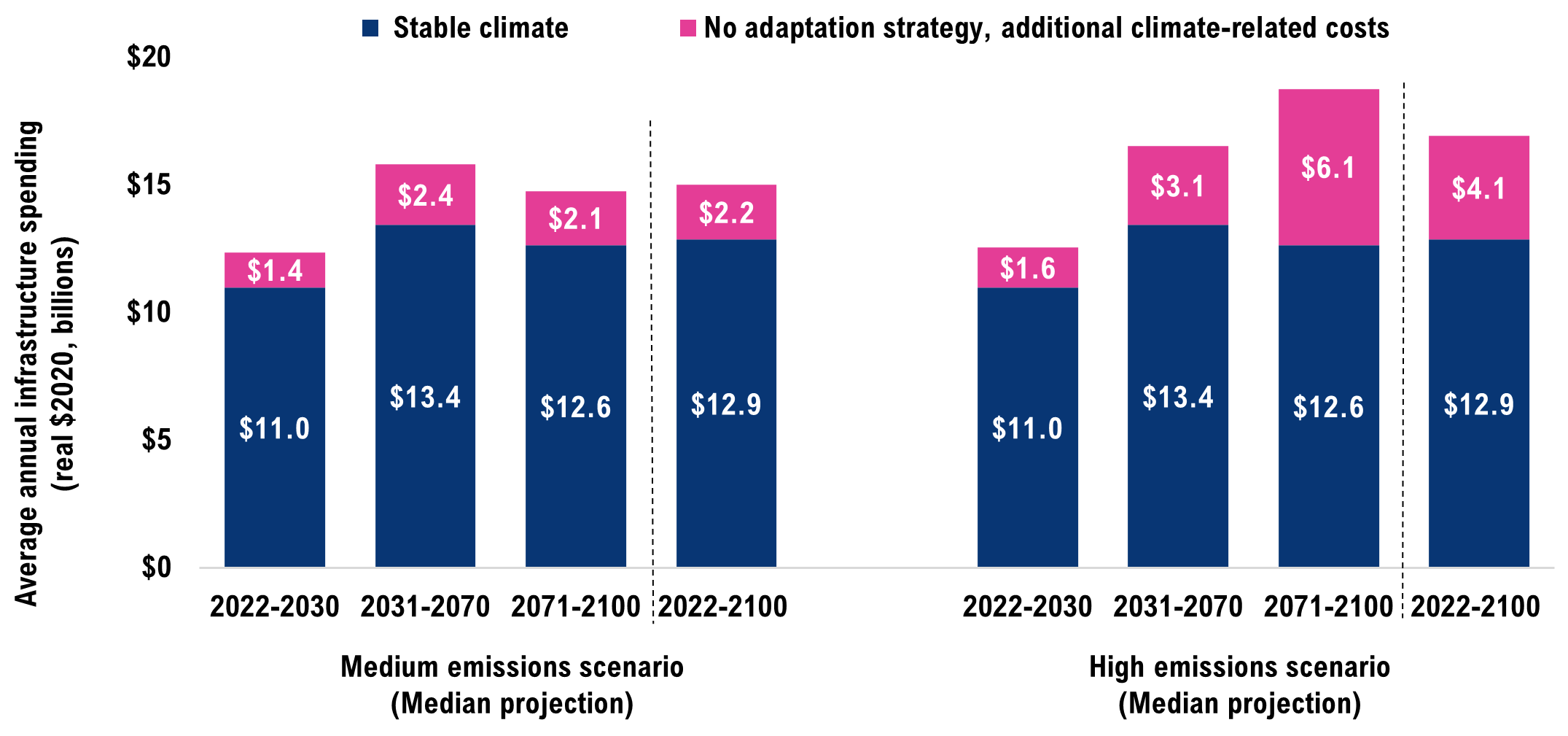
Note: Uncertainty ranges are omitted from this chart for presentation purposes.
Source: FAO.
In the high emissions scenario (median projection), average annual infrastructure costs would instead increase by $4.1 billion per year over the century, a 32 per cent increase in costs relative to the stable climate scenario. In this case, climate-related costs increase from $1.6 billion this decade, to an average of $3.1 billion in the mid-century period, and continue rising to $6.1 billion by late century. This occurs due to the continued deterioration of climate hazards in the high emissions scenario.
Figure 4-5 Uncertainty ranges around annual climate-related costs widen over time
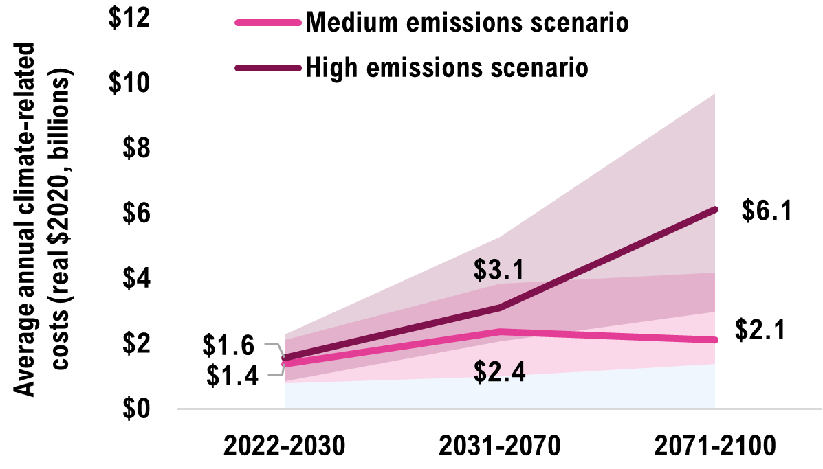
Source: FAO.
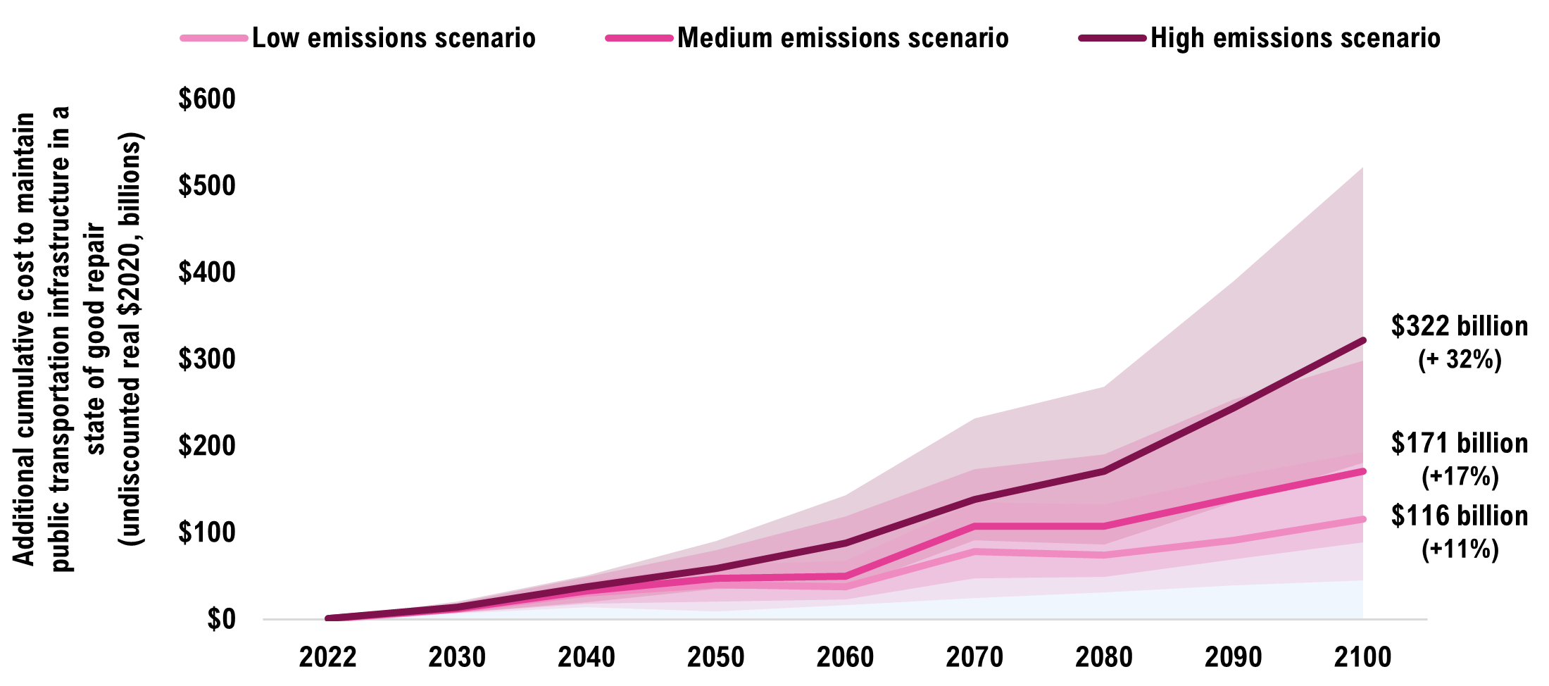
Figure 4-6 In the absence of adaptation, climate-related costs accumulate to significant sums by 2100
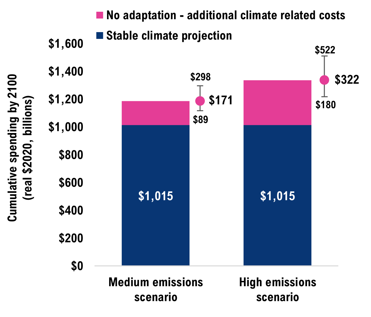
Source: FAO.
There is uncertainty in the extent of warming that will occur in each emissions scenario (see Page 17), as well as engineering uncertainty in how changing climate hazards will impact Ontario’s infrastructure (see Appendix C). The full range of average annual climate-related costs is presented in Figure 4-5.
These average annual costs would cumulate over the projection. In the short term, changing climate hazards are already adding to the cost of maintaining public transportation infrastructure. Annual climate-related costs across the medium and high emissions scenarios average $1.5 billion from 2022-2030, which would accumulate to approximately $13.3 billion by 2030 in the absence of adaptation.[30] This is a 13 per cent increase in provincial and municipal infrastructure costs relative to the stable climate projection.
In the medium emissions scenario (median projection), the cumulative cost of maintaining the existing portfolio of public transportation infrastructure in a state of good repair will increase by $171 billion over the century.This represents a 17 per cent increase in costs over what would have occurred in a stable climate. These cumulative costs could range from $89 billion to $298 billion given the climate and engineering uncertainties.
In the high emissions scenario (median projection), the cumulative cost would instead increase by $322 billion (a 32 per cent increase), with a range of $180 billion to $522 billion.
5 | Adapting public transportation infrastructure to climate hazards
Chapter 4 described the financial impact of not adapting public transportation infrastructure to the projected changes in extreme rainfall, extreme heat and freeze-thaw cycles. In practice, transportation infrastructure can be adapted to withstand these impacts – ensuring that assets perform to the same standards for which they were initially designed and avoiding accelerated deterioration or higher O&M expenses.
This chapter discusses different forms of adaptation, defines the scope of adaptation analyzed in this report, and estimates a range of costs to adapt Ontario’s portfolio of public transportation infrastructure to withstand the late-century climate projections for extreme rainfall and extreme heat in the medium and high emissions scenarios.[31]
Adapting public transportation infrastructure can help prevent the impacts of climate hazards
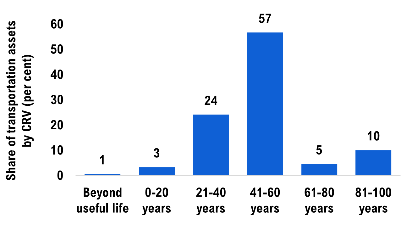
Figure 5-1 Ontario’s public transportation infrastructure assets have long remaining useful lives
Source: FAO.
Ontario’s public transportation infrastructure assets have long useful lives. Of the $330 billion in infrastructure, nearly 72 per cent has a remaining useful life of more than 40 years. Given the long useful lives of public transportation infrastructure assets, late-century climate conditions are relevant to adaptation decisions being made now. These decisions will impact public infrastructure costs throughout the century.
However, climate projections depend on the trajectory of global emissions, which remains uncertain. This raises the difficult question of how projected changes in key climate hazards should be accounted for when public transportation infrastructure is designed, built or retrofitted.[32]
Adapting transportation infrastructure to changing climate hazards could take many forms. A few examples include:
- updating infrastructure design parameters to a higher standard, including those detailed in the Canadian Highway Bridge Design Code;[33]
- using Intensity-Duration-Frequency tools that project future rainfall intensities for the design and replacement of transportation infrastructure;[34]
- using pavement mixes for roads with higher heat tolerance;[35]
- expanding the drainage capacity of culverts;[36]
- using thermosyphons to maintain permafrost stability and improve northern road and highway performance;[37] and
- changing the way assets are managed, for example, altering the frequency of operations and maintenance schedules.[38]
In the FAO’s framework, adaptation is modelled as an alteration of the physical components of transportation infrastructure to prevent damage costs caused by changing climate hazards.[39] Figure 5‑2 presents some examples of adaptation measures for transportation infrastructure components.[40]
Figure 5-2 Examples of transportation infrastructure adaptations to climate hazards
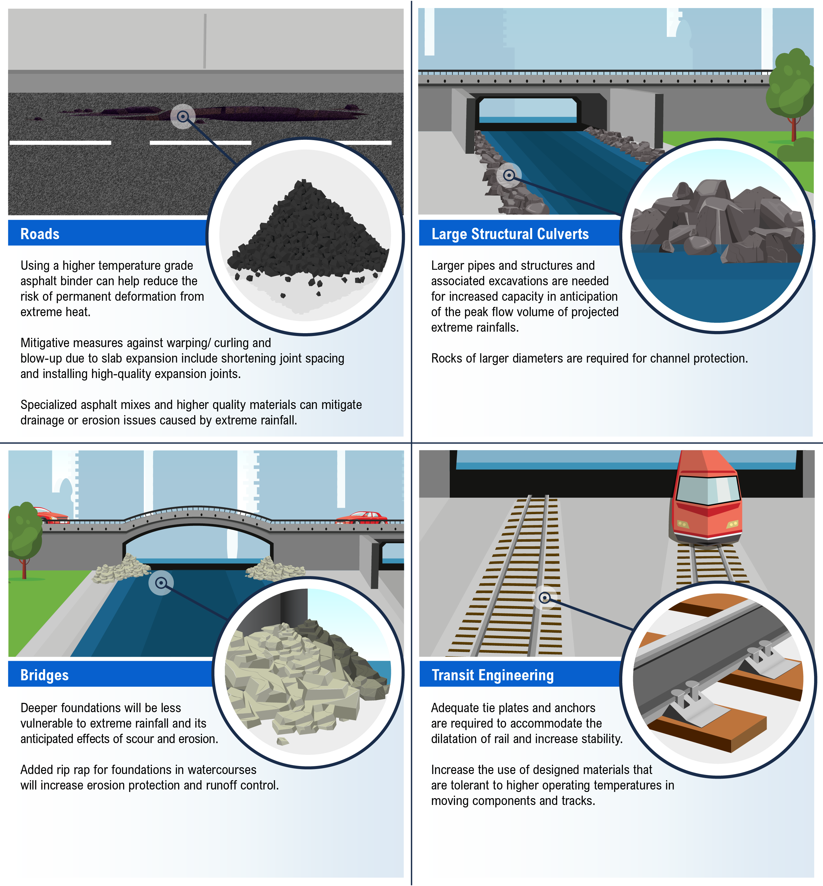
Note: For more examples of how transportation infrastructure components can be adapted to climate hazards, see WSP 2021.
Source: WSP.
Adaptation strategy costs vary based on the approach taken
To estimate adaptation costs, the FAO assumed that public transportation infrastructure is adapted at the time of rehabilitation or renewal to withstand the late-century projections[41] of each climate hazard.[42] Once an asset is adapted, the FAO assumes that it no longer faces additional O&M and capital expenses due to changing climate hazards.[43] However, since adaptation increases the value of an asset, its post-adaptation O&M and capital expenses also increase, reflecting its higher value.
The additional infrastructure costs of an adaptation strategy include: higher capital expenses from increased deterioration and higher O&M expenses until adaptation, a one-time adaptation expense (either through a retrofit or renewal), and higher O&M and capital expenses required to maintain higher-valued adapted assets. The costs presented in this chapter would occur instead of those estimated in the no adaptation strategy presented in Chapter 4.
The costs of an adaptation strategy would vary based on when the adaptation actions are undertaken. To highlight how the costs could vary, the FAO developed two adaptation strategies.
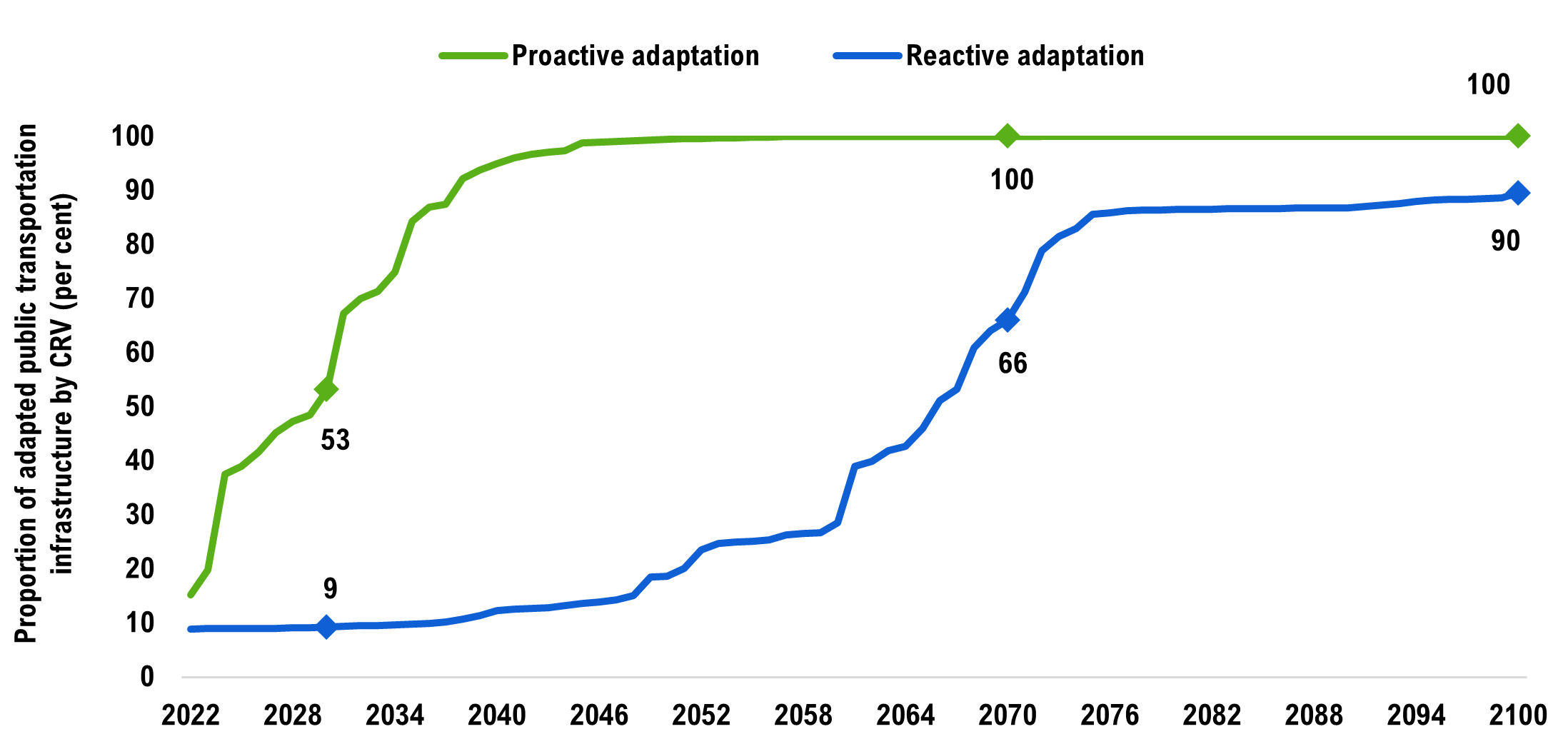
- Reactive adaptation strategy: Transportation assets are only adapted at the time of renewal. This approach results in a gradual increase in the share of adapted assets over the century, with roughly 90 per cent of assets adapted by 2100. The remaining 10 per cent have service lives that extend beyond 2100 and are not renewed or adapted over the projection.
- Proactive adaptation strategy: Transportation assets are adapted at the first available opportunity. This occurs either during an asset’s next major rehabilitation through a retrofit[44] or at renewal, whichever comes first. In this approach, all transportation assets are adapted by the 2050s.
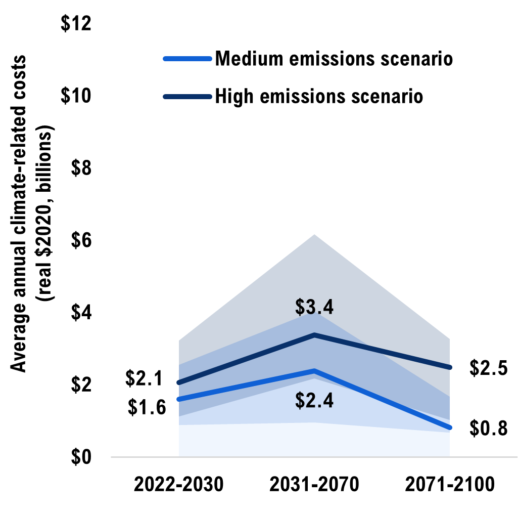
Figure 5-3 The reactive adaptation strategy leaves most public transportation assets vulnerable to changing climate hazards throughout the mid-century.
Source: FAO.
Projecting public transportation infrastructure costs in the reactive adaptation strategy
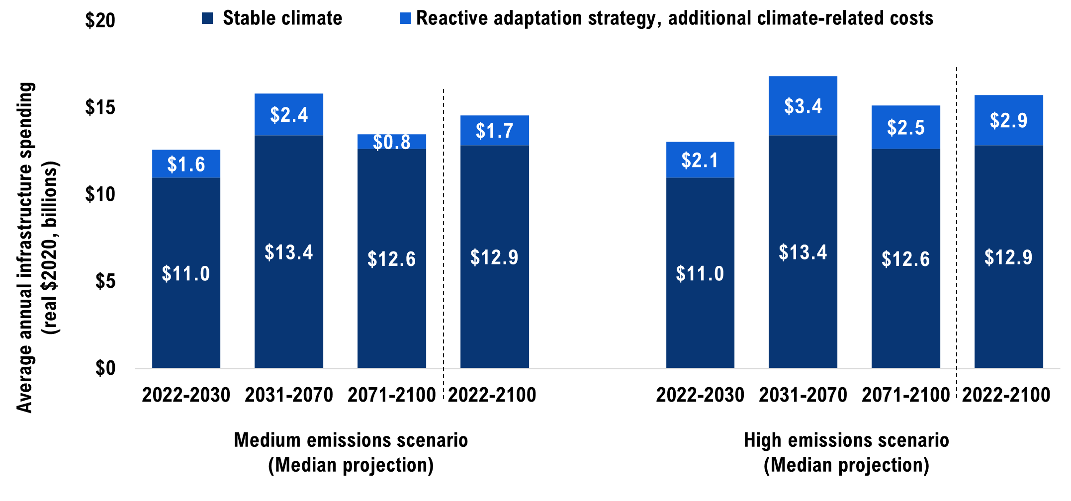
In the medium emissions scenario (median projection), the average annual cost of maintaining the existing portfolio of public transportation infrastructure in a state of good repair will increase by $1.7 billion per year over the century.This represents a 13 per cent increase in costs over what would have occurred in a stable climate. These average annual costs fluctuate from $1.6 billion per year this decade, to $2.4 billion in the mid-century period as the share of adapted assets rises from nine per cent in 2030 to 66 per cent in 2070. By late century, these costs decline to $0.8 billion per year as adapted public transportation assets avoid damage costs associated with late century climate conditions (see Figure 5-3).
In the high emissions scenario (median projection), average annual infrastructure costs would instead increase by $2.9 billion per year over the century, a 23 per cent increase in costs relative to the stable climate scenario. In this case, climate-related costs increase from $2.1 billion this decade, to an average of $3.4 billion in the mid-century period, then declining to $2.5 billion in the late century period. Costs in this scenario reflect higher damage costs from more extreme climate hazards, as well as higher adaptation costs to enable public transportation infrastructure to withstand these hazards.
Figure 5-4 Adaptation will raise transportation infrastructure costs, but more so in the high emissions scenario
Note: Uncertainty ranges are omitted from this chart for presentation purpose.
Source: FAO
Figure 5-5 Climate-related costs are subject to climate and engineering uncertainty
Source: FAO.
Given the uncertain extent of warming that will occur in each emissions scenario, as well as the engineering uncertainty in costing the array of adaptation options, the full range of climate-related costs is presented in Figure 5-5.
These projected annual costs will accumulate over the remainder of this century. In the first decade of the reactive adaptation strategy, approximately nine per cent of public transportation assets are adapted, while the remaining assets continue to incur damage costs.
The FAO projects that these climate-related costs would accumulate to approximately $14 billion by 2030 in the medium emissions scenario (a 15 per cent increase in provincial and municipal infrastructure costs relative to the stable climate projection), or approximately $19 billion by 2030 in the high emissions scenario (a 19 per cent increase).[45]
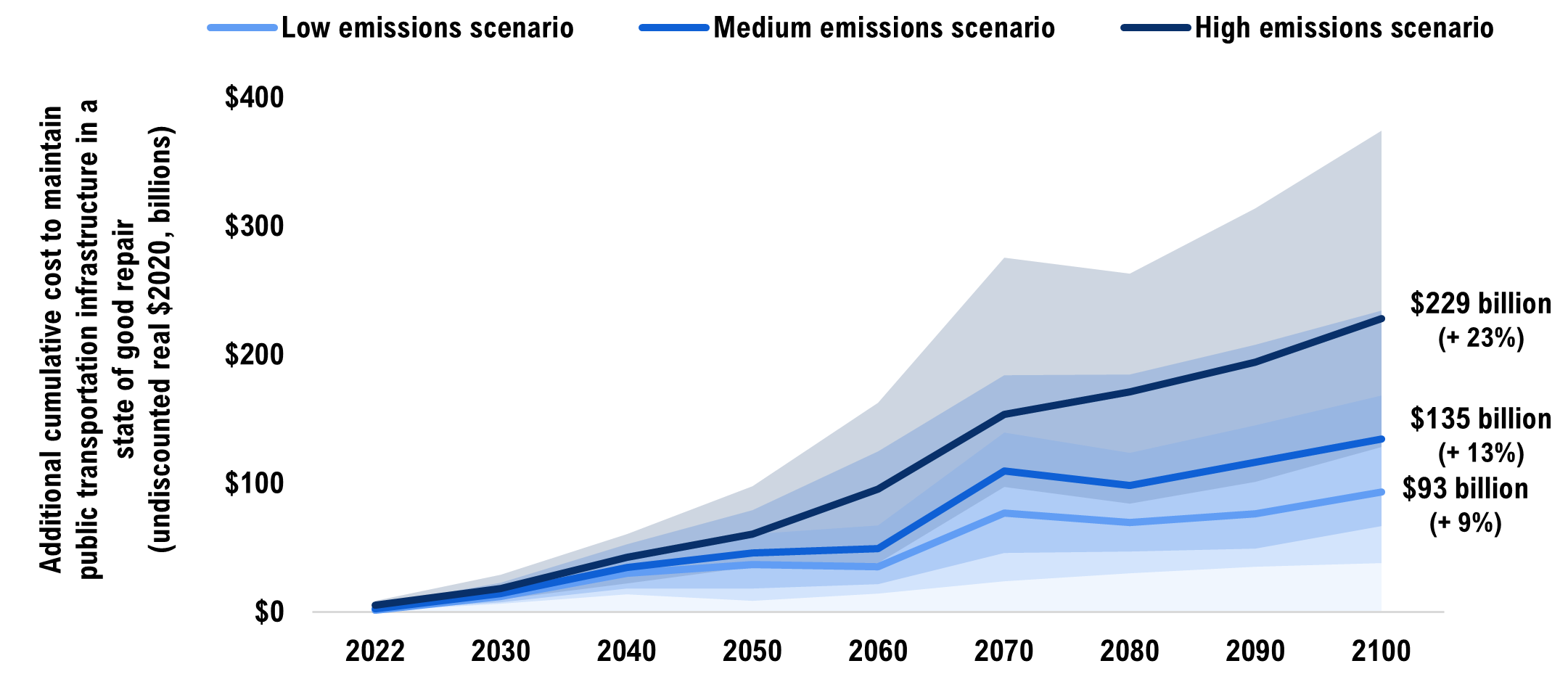
Figure 5-6 Cumulative climate-related costs in the reactive adaptation strategy to 2100
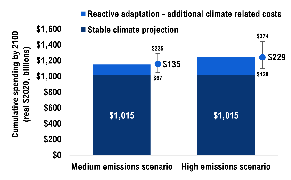
Source: FAO.
In the medium emissions scenario (median projection), the cumulative cost of maintaining the existing portfolio of public transportation infrastructure in a state of good repair will increase by $135 billion over the century.This represents a 13 per cent increase in costs over what would have occurred in a stable climate. These cumulative costs could range from $67 billion to $235 billion given the climate and engineering uncertainties.
In the high emissions scenario (median projection), the cumulative cost would instead increase by $229 billion (a 23 per cent increase), with a range of $129 billion to $374 billion.
Projecting public transportation infrastructure costs in the proactive adaptation strategy
In the proactive adaptation strategy,transportation assets are adapted at the first available opportunity. It is assumed that over 50 per cent of infrastructure assets are adapted by 2030 and 100 per cent are adapted by 2070 (see Figure 5-3).
In the medium emissions scenario (median projection), the average annual cost of maintaining the existing portfolio of public transportation infrastructure in a state of good repair will increase by $1.4 billion per year over the century.This represents an 11 per cent increase in costs over what would have occurred in a stable climate. These average annual costs decline from $2.9 billion per year this decade (when over half of public transportation assets are assumed to be adapted), to $1.4 billion in the mid-century period, and to $1.0 billion per year by late century, as adapted public transportation assets avoid damage costs associated with late century climate conditions (see Figure 5-7).
In the high emissions scenario (median projection), average annual infrastructure costs would instead increase by $2.7 billion per year over the century, a 21 per cent increase in costs relative to the stable climate scenario. In this case, climate-related costs decline from $5.2 billion per year this decade, to an average of $2.8 billion in the mid-century period, then declining to $2.0 billion in the late century period. Costs in this scenario reflect higher damage costs from more extreme climate hazards, as well as higher adaptation costs to enable public transportation infrastructure to withstand these hazards.
Figure 5-7 Adaptation will raise transportation infrastructure costs, but more so in the high emissions scenario
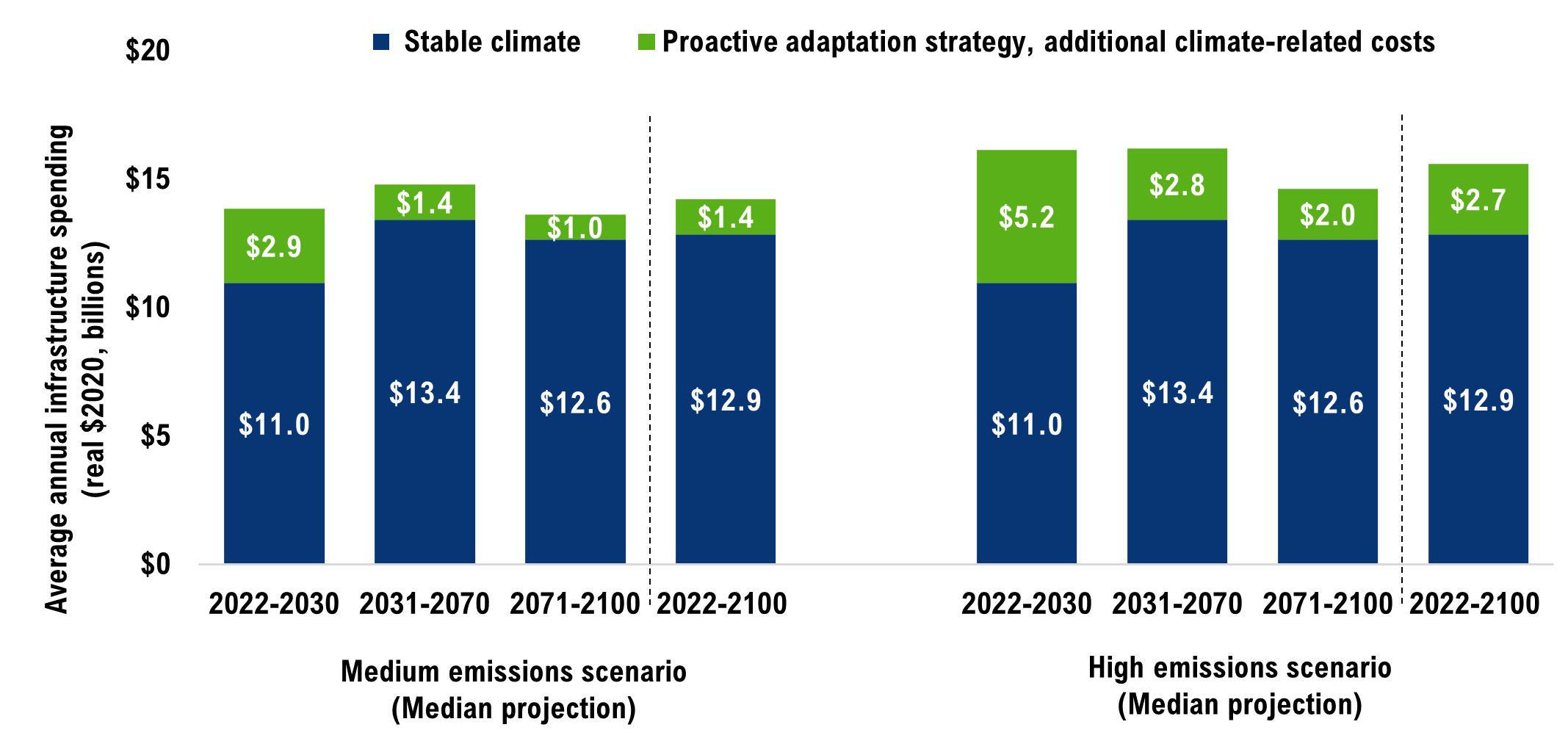
Note: Uncertainty ranges are omitted from this chart for presentation purpose.
Source: FAO
Figure 5-8 Climate-related costs are subject to climate and engineering uncertainty
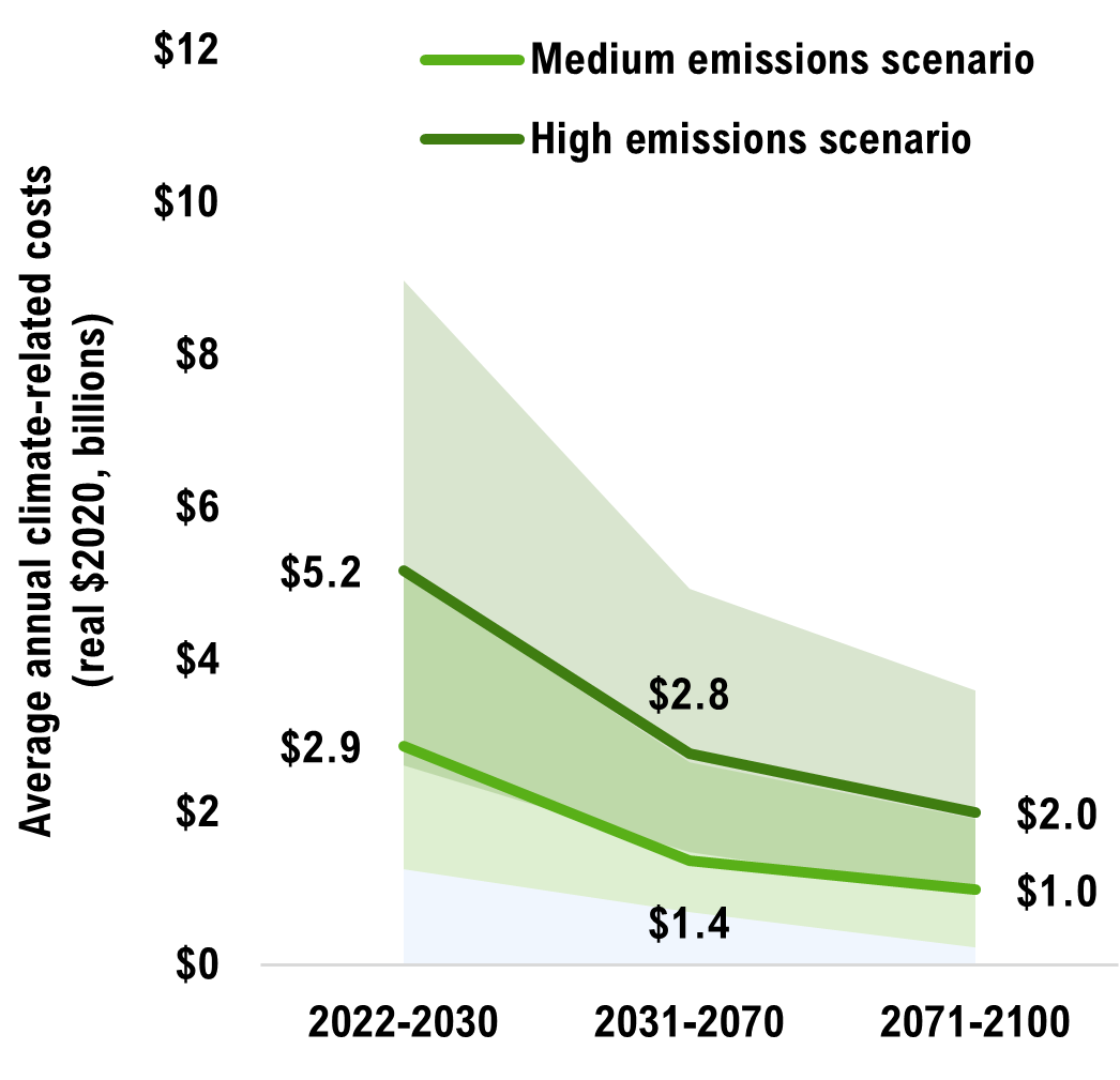
Source: FAO.
However, given the uncertain extent of warming that will occur in each emissions scenario, as well as the engineering uncertainty in costing the array of adaptation options, the full range of annual climate-related costs is presented in Figure 5-8.
In the first decade of the proactive adaptation strategy, approximately 53 per cent of public transportation assets are assumed to be adapted, while the remaining assets continue to incur damage costs.
The FAO projects that these climate-related costs would accumulate to approximately $26 billion by 2030 in the medium emissions scenario(a 26 per cent increase in provincial and municipal infrastructure costs relative to the stable climate projection), or approximately $47 billion by 2030 in the high emissions scenario (a 47 per cent increase).[46]
Figure 5-9 Cumulative climate-related costs in the proactive adaptation strategy to 2100
Source: FAO.
In the medium emissions scenario (median projection), the cumulative cost of maintaining the existing portfolio of public transportation infrastructure in a state of good repair will increase by $110 billion over the century.This represents an 11 per cent increase in costs over what would have occurred in a stable climate. These cumulative costs could range from $46 billion to $210 billion given the climate and engineering uncertainties.
In the high emissions scenario (median projection), the cumulative cost would instead increase by $217 billion (a 21 per cent increase), with a range of $111 billion to $386 billion.
6 | Comparing different asset management strategies
Chapters 4 and 5 examined the costs of maintaining public transportation infrastructure in a state of good repair in the presence of climate change under three asset management strategies: no adaptation, reactive adaptation and proactive adaptation. None of the strategies presented in this report are meant to be a precise representation of future costs, and the portfolio level costing results are not intended to inform asset-specific management decisions. These strategies were designed to estimate the scale of the budgetary impact that changes in extreme rainfall, extreme heat and freeze-thaw cycles will impose on the Province and municipalities over the rest of the century.
This chapter compares cost estimates across the three asset management strategies and discusses the difference in cost profiles between them. The chapter then discusses the factors that were beyond the scope of the FAO’s analysis but are relevant in determining the most cost-effective strategy for managing Ontario’s public transportation infrastructure in a changing climate.
Adapting public transportation infrastructure is less expensive than not adapting over the long term
The financial impact of extreme rainfall, extreme heat and freeze-thaw cycles will be material to the Province and municipalities regardless of which asset management strategy is pursued. However, the FAO estimates that on an undiscounted basis, the cumulative costs by the end of the 21st century are the highest under the no adaptation strategy and lowest under the proactive adaptation strategy under both emissions scenarios. For a discussion of these cost profiles on a discounted basis, see Appendix D.
Figure 6-1 shows that the future path of global climate change will influence the extent of additional climate-related infrastructure costs, which are much lower in the medium emissions scenario than in the high emissions scenario (median projections) across all asset management strategies.
Figure 6-1 Adapting Ontario’s public transportation infrastructure will cost Provincial and municipal governments less than not adapting in a changing climate
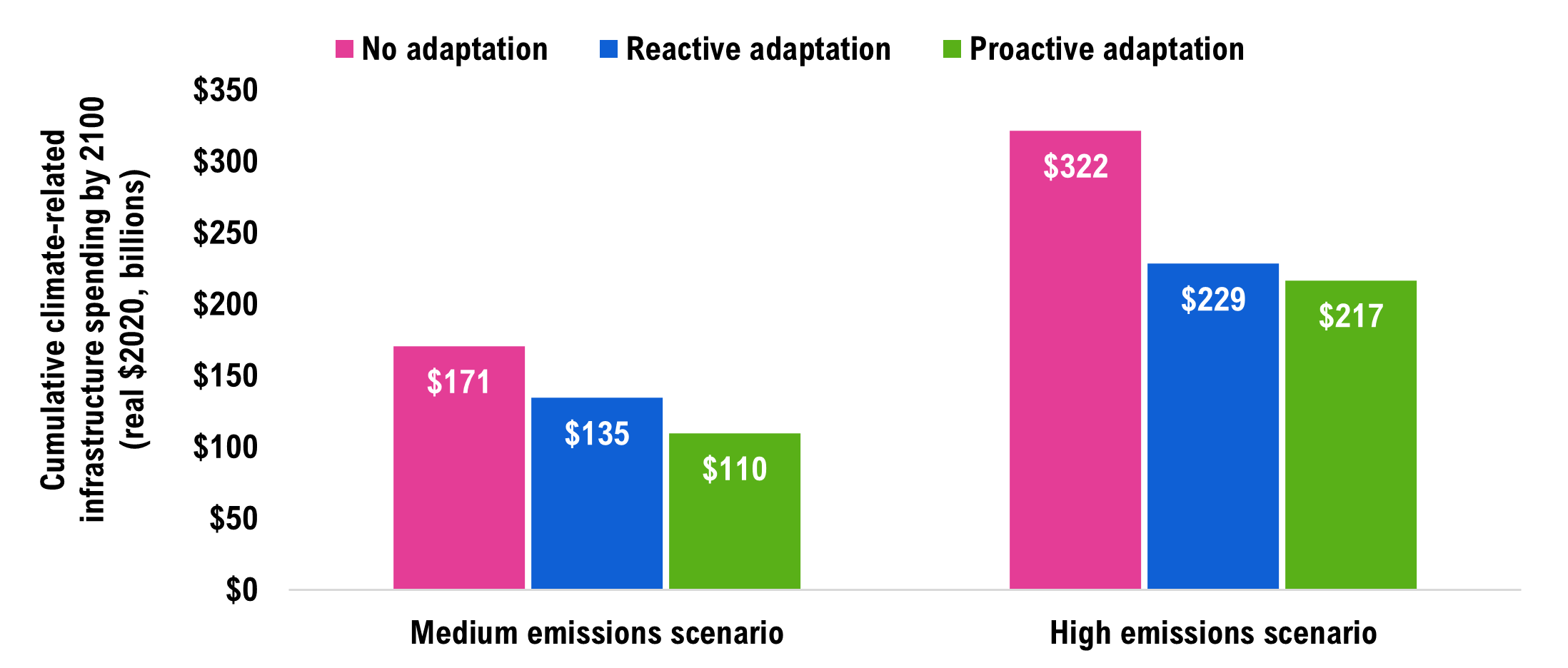
Note: The costs in this chart are based on the median (or 50th percentile) projection under each emissions scenario and are in addition to the baseline costs over the same period. Uncertainty ranges are omitted from this chart for presentation purpose.
Source: FAO.
Proactively adapting public transportation infrastructure requires higher upfront costs but rapidly reduces climate vulnerability
Figure 6-2 shows how costs accumulate in the medium and high emissions scenarios (median projections) under the three asset management strategies.
Figure 6-2 The three asset management strategies have different cost profiles
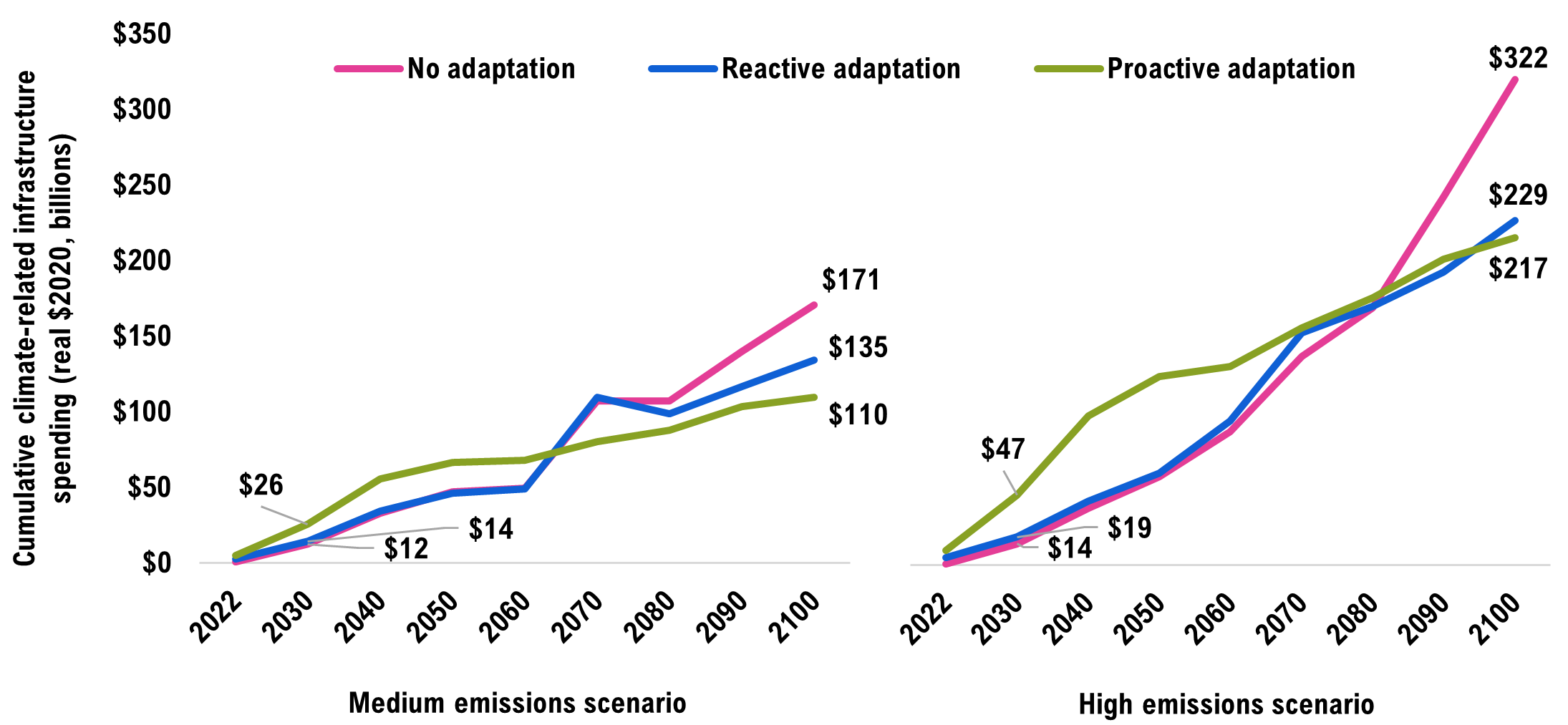
Note: The costs in this chart are based on the median (or 50th percentile) projection under each emissions scenario and are in addition to the baseline costs over the same period. Uncertainty ranges are omitted from this chart for presentation purpose.
Source: FAO.
In the first half of the century, the cost profiles of the no adaptation strategy and the reactive adaptation strategyare similar, as damage costs from worsening climate hazards are incurred in both strategies. These costs profiles diverge in the second half of the century as the impact of more frequent and intense climate hazards becomes more costly in the no adaptation strategy, whereas these costs are avoided in the reactive adaptation strategy since over 66 per cent of public transportation assets are adapted by 2070 (see Figure 5-3).
The proactive adaptation strategy sees a substantial accumulation in costs over the next four decades as all assets are adapted by the 2050s, rapidly reducing the vulnerability of Ontario’s transportation infrastructure to these changing climate hazards. The result is a much slower accumulation of costs in the second half of the century, as climate damages are avoided. By the end of the century, the proactive adaptation strategy results in the lowest cumulative additional costs of the three strategies in real 2020 dollars.
Costs to households and businesses should be included in assessing the cost-effectiveness of adaptation action
This report accounts for the direct infrastructure costs to government but excludes any costs to households or businesses from infrastructure service disruptions. For example, if a municipal road becomes damaged and must be repaired, this analysis includes only the cost of those repairs to the municipality, not the costs to households and businesses of traffic delays.[47]
Examples of costs to households and businesses include the following:
- Traffic congestion occurs during the rehabilitation and renewal of transportation assets, slowing travel times and impacting productivity. For example, a recent Canadian Climate Institute study of the climate impacts to public infrastructure states that: “…the costs of delays and travel disruptions on road and rail systems could be nearly as high as the costs of direct physical damage to the infrastructure itself.”[48]
- Beyond the delay costs, climate-related disruptions to transportation networks would impact supply chains, the labour market and the economy more broadly.[49]
- Climate-related disruptions to transportation networks also have non-financial costs, including increased response times to health and environmental emergencies,[50] or higher risks of being cut off from vital services in rural and remote communities.
Costing these broader societal impacts was beyond the scope of this report. These costs are likely to be material and if added, would likely show further benefits of adapting public transportation infrastructure. Estimating these impacts would be a useful area of future research.
Making asset-specific adaptation decisions should consider many other factors
Costing three different asset management strategies at the portfolio level was designed to estimate the scale of the budgetary impact that changes in extreme rainfall, extreme heat and freeze-thaw cycles could impose over the rest of the century. However, to make asset-specific climate adaptation decisions, many other factors should be considered,[51] including:
- an asset’s individual characteristics (including age, condition and specific climate vulnerabilities);
- a wider array of climate impacts over the entire useful life of an asset;
- costs to households and businesses; and
- non-asset related considerations, including surrounding infrastructure. For example, if a section of stormwater pipe located underneath a road is being replaced (or adapted), adapting the road may also be considered.
Incorporating these factors would further enhance the FAO’s methodology and would better support adaptation decision-making for individual assets in a changing climate.
7 | Appendix
Appendix A: Scope of transportation sector assets analyzed
| Level of Government | Sector | Total CRV (2020$ billions) | Description |
|---|---|---|---|
| Provincial | Roads | $19 |
|
| Bridges | $23 |
|
|
| Large Structural Culverts (>3 metres) | $5 |
|
|
| Transit Engineering | $13 |
|
|
| Municipal | Roads | $221 |
|
| Bridges | $35 |
|
|
| Large Structural Culverts (>3 metres) | $7 |
|
|
| Transit Engineering | $6 |
|
Appendix B: Scope of climate variables used in costing analysis
The Canadian Centre for Climate Services provided the projections of all climate indicators used in the FAO’s costing analysis. Depending on the nature of the hazard’s interaction with specific transportation infrastructure components, different climate indicators were used. See WSP’s report for a full description and rationale.[52]
| Climate Hazard | Variable | Definition | Low Emissions (RCP2.6) | Medium Emissions (RCP4.5) | High Emissions (RCP8.5) |
|---|---|---|---|---|---|
| Extreme Heat | Annual number of hot days | Annual number of days with daily maximum temperature above 30°C | +6 days or +138.9% (+2 to 10 days or +64.2 to 223.1%) | +13 days or +336.5% (+6 to 18 days or +167.8 to 422.0%) | +34 days or +860.7% (+17 to 46 days or +493.8 to 1050.6%) |
| Extreme Rainfall | IDF 24-hour 1:100 | Short duration rainfall intensity for a 24-hour 1-in-100-year event | +14.6% (+9.8 to 23.5%) | +24.9% (+16.1 to 39.4%) | +53.0% (+38.0 to 78.2%) |
| Freeze-Thaw Cycles | Annual freeze-thaw cycles | Annual number of days with daily maximum temperature above 0°C and daily minimum temperature below 0°C | -5.5% (-15.2 to 0.0%) | -12.1% (-19.2 to 0.0%) | -15.1% (-24.9 to 0.0%) |
The full suite of climate data used in the CIPI project is available at the CIPI section of the FAO’s website.
Appendix C: The impact of changing climate hazards on key transportation infrastructure costs
This appendix presents the impact of climate hazards on the key infrastructure costs for roads, bridges, large structural culverts and transit engineering assets. First, the appendix presents the total impact of the climate hazards considered in this study on the useful service life (USL) and operations and maintenance (O&M) spending in the absence of adaptation, as well as the costs of retrofit and renewal adaptation to prevent these climate damages. Next, the appendix presents a detailed breakdown of the impact of each climate hazard on O&M spending and USL by asset type.
To establish relationships between relevant climate indicators and key infrastructure costs, the FAO worked with WSP, a large engineering firm with expertise in all aspects of public sector infrastructure, including asset management, public infrastructure construction and operations, and climate change impacts.
The FAO and WSP first established which of the three climate hazards could have the most significant impact, and on which asset type. As each hazard would interact with each asset-type in a different way, it was agreed that WSP would focus attention on the “interactions” that could present the greatest financial impact to asset managers. For example, while extreme heat may impact bridges, because the impact of extreme rainfall and freeze-thaw cycles was deemed more important, only these hazards were examined.
WSP estimated relationships between changing climate variables and infrastructure costs by surveying relevant engineering experts. To account for engineering uncertainty, WSP aggregated its responses and provided optimistic, pessimistic and most-likely cost relationships.[53] This forms the basis on which the FAO estimated the additional costs of climate hazards to public transportation infrastructure in Ontario.[54]
While regional climate projections were used to develop the FAO’s infrastructure cost estimates, for simplicity, this appendix presents Ontario-average infrastructure cost results by asset type. The results reflect a weighted average climate projection based on the proportion of assets (by CRV) located in each region.[55] The charts below provide three estimates for each infrastructure cost impact in the medium and high emissions scenarios:
- The solid lines represent the most likely infrastructure cost impact for the 50th percentile climate projection.
- The upper limit of the uncertainty bands represents the pessimistic infrastructure cost impact for the 90th percentile climate projection.
- The lower limit of the uncertainty bands represents the optimistic infrastructure cost impacts of the 10th percentile climate projection.
| In Absence of Adaptation | |
|
Useful Service Life 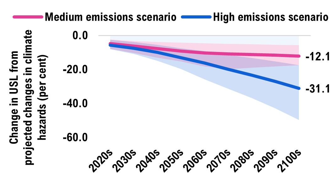
|
|
|
Operations & Maintenance 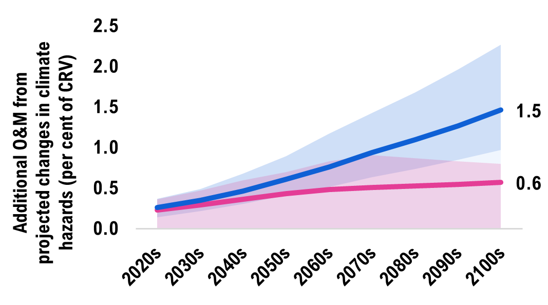
|
|
| Adaptation Costs | |
|
Retrofit Costs 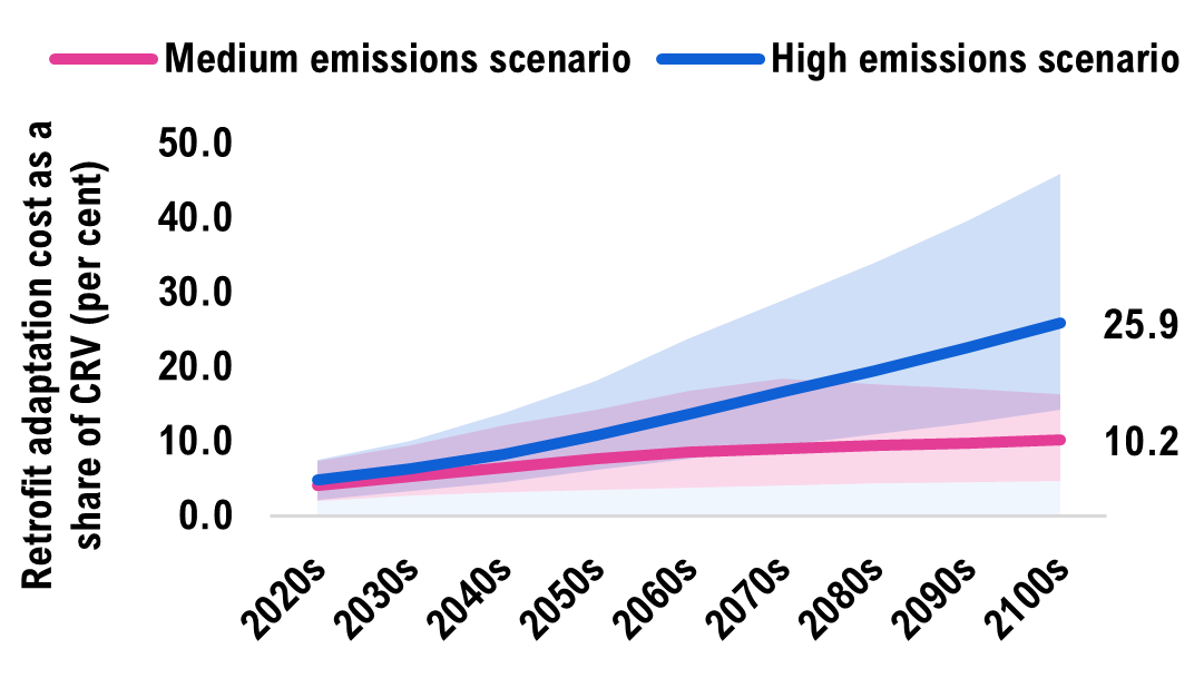
|
|
|
Renewal Costs 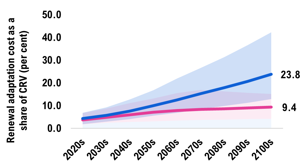
|
|
Accessible version
| In Absence of Adaptation | ||||||||||
|---|---|---|---|---|---|---|---|---|---|---|
| Useful Service Life | ||||||||||
| Emissions Scenario | 2020s | 2030s | 2040s | 2050s | 2060s | 2070s | 2080s | 2090s | 2100s | |
| Medium | Low | -2.4 | -3.2 | -3.8 | -4.2 | -4.6 | -5.0 | -5.2 | -5.4 | -5.7 |
| Median | -4.8 | -6.2 | -7.7 | -9.2 | -10.2 | -10.8 | -11.2 | -11.7 | -12.1 | |
| High | -7.9 | -10.2 | -13.1 | -15.3 | -18.2 | -19.9 | -19.0 | -18.2 | -17.5 | |
| High | Low | -2.5 | -3.9 | -5.5 | -7.5 | -9.3 | -11.4 | -13.2 | -15.2 | -17.4 |
| Median | -5.6 | -7.5 | -9.9 | -13.0 | -16.2 | -19.9 | -23.3 | -27.0 | -31.1 | |
| High | -8.0 | -10.8 | -14.9 | -19.6 | -25.7 | -31.2 | -36.9 | -43.0 | -49.7 | |
| Operations & Maintenance | ||||||||||
| Emissions Scenario | 2020s | 2030s | 2040s | 2050s | 2060s | 2070s | 2080s | 2090s | 2100s | |
| Medium | Low | 0.1 | 0.2 | 0.2 | 0.2 | 0.3 | 0.3 | 0.3 | 0.3 | 0.3 |
| Median | 0.2 | 0.3 | 0.4 | 0.4 | 0.5 | 0.5 | 0.5 | 0.5 | 0.6 | |
| High | 0.4 | 0.5 | 0.6 | 0.7 | 0.8 | 0.9 | 0.9 | 0.8 | 0.8 | |
| High | Low | 0.1 | 0.2 | 0.3 | 0.4 | 0.5 | 0.6 | 0.7 | 0.8 | 1.0 |
| Median | 0.3 | 0.4 | 0.5 | 0.6 | 0.8 | 0.9 | 1.1 | 1.3 | 1.5 | |
| High | 0.4 | 0.5 | 0.7 | 0.9 | 1.2 | 1.4 | 1.7 | 2.0 | 2.3 | |
| Adaptation Costs | ||||||||||
| Retrofit Costs | ||||||||||
| Emissions Scenario | 2020s | 2030s | 2040s | 2050s | 2060s | 2070s | 2080s | 2090s | 2100s | |
| Medium | Low | 2.0 | 2.7 | 3.2 | 3.4 | 3.8 | 4.1 | 4.3 | 4.5 | 4.7 |
| Median | 4.1 | 5.2 | 6.5 | 7.7 | 8.6 | 9.0 | 9.4 | 9.8 | 10.2 | |
| High | 7.3 | 9.5 | 12.1 | 14.2 | 16.8 | 18.3 | 17.7 | 17.0 | 16.4 | |
| High | Low | 2.1 | 3.2 | 4.5 | 6.1 | 7.6 | 9.4 | 10.9 | 12.5 | 14.2 |
| Median | 4.7 | 6.3 | 8.3 | 10.9 | 13.6 | 16.6 | 19.5 | 22.5 | 25.9 | |
| High | 7.5 | 10.0 | 13.8 | 18.1 | 23.7 | 28.8 | 34.0 | 39.7 | 45.8 | |
| Renewal Costs | ||||||||||
| Emissions Scenario | 2020s | 2030s | 2040s | 2050s | 2060s | 2070s | 2080s | 2090s | 2100s | |
| Medium | Low | 1.8 | 2.4 | 2.9 | 3.1 | 3.5 | 3.7 | 3.9 | 4.1 | 4.3 |
| Median | 3.8 | 4.8 | 6.0 | 7.1 | 7.9 | 8.3 | 8.7 | 9.0 | 9.4 | |
| High | 6.8 | 8.8 | 11.2 | 13.1 | 15.5 | 16.9 | 16.3 | 15.7 | 15.1 | |
| High | Low | 1.9 | 2.9 | 4.1 | 5.6 | 6.9 | 8.5 | 9.8 | 11.3 | 12.9 |
| Median | 4.4 | 5.8 | 7.6 | 10.0 | 12.5 | 15.3 | 17.9 | 20.8 | 23.8 | |
| High | 6.9 | 9.2 | 12.7 | 16.7 | 21.9 | 26.6 | 31.4 | 36.6 | 42.3 | |
| In Absence of Adaptation | |
|
Useful Service Life 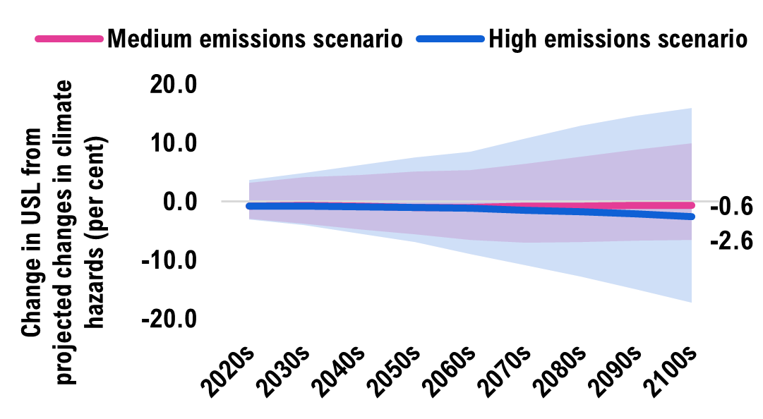
|
|
|
Operations & Maintenance 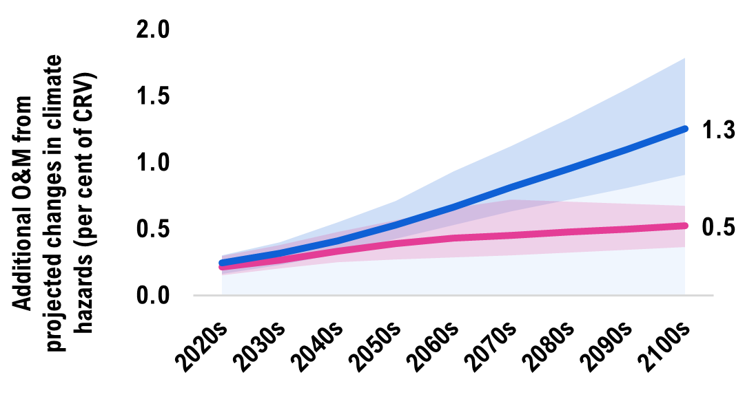
|
|
| Adaptation Costs | |
|
Retrofit Costs 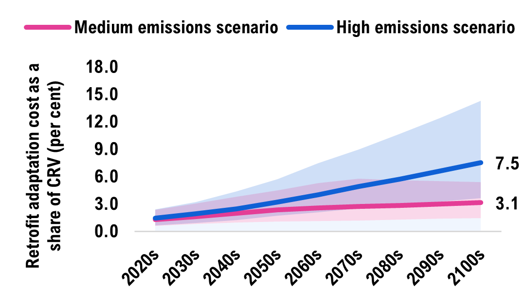
|
|
|
Renewal Costs 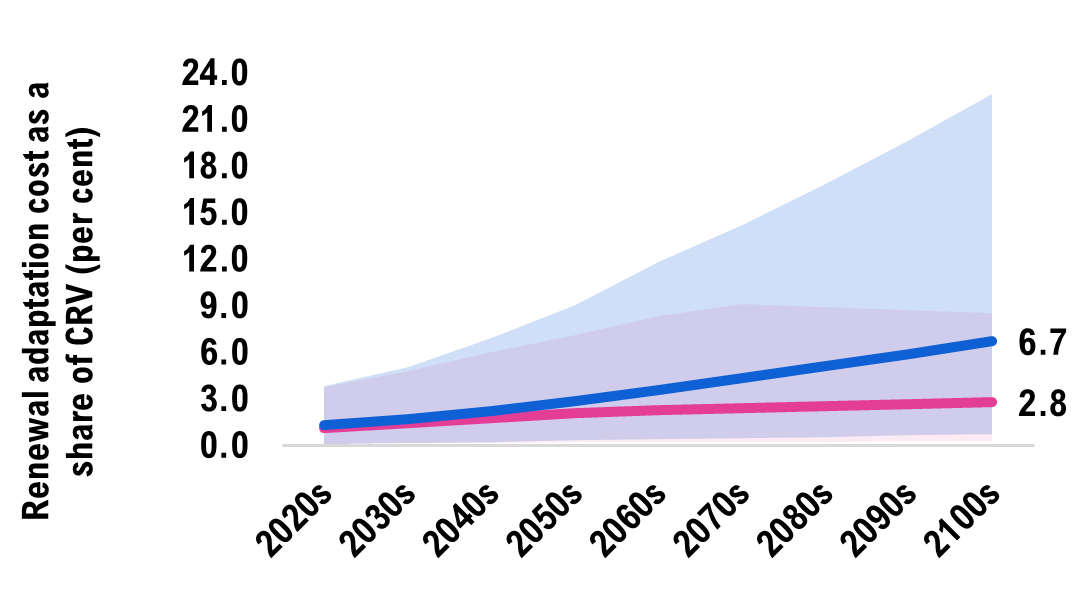
|
|
Accessible version
| In Absence of Adaptation | ||||||||||
|---|---|---|---|---|---|---|---|---|---|---|
| Useful Service Life | ||||||||||
| Emissions Scenario | 2020s | 2030s | 2040s | 2050s | 2060s | 2070s | 2080s | 2090s | 2100s | |
| Medium | Low | 3.3 | 4.2 | 4.5 | 5.1 | 5.4 | 6.5 | 7.7 | 8.9 | 9.9 |
| Median | -0.7 | -0.7 | -0.8 | -0.9 | -0.9 | -0.8 | -0.7 | -0.6 | -0.6 | |
| High | -3.0 | -3.7 | -4.7 | -5.6 | -6.5 | -7.0 | -6.9 | -6.7 | -6.5 | |
| High | Low | 3.7 | 4.9 | 6.3 | 7.5 | 8.5 | 10.9 | 12.9 | 14.6 | 16.0 |
| Median | -0.7 | -0.7 | -0.9 | -1.0 | -1.1 | -1.4 | -1.7 | -2.1 | -2.6 | |
| High | -3.0 | -3.9 | -5.4 | -6.9 | -9.0 | -10.8 | -12.8 | -14.9 | -17.2 | |
| Operations & Maintenance | ||||||||||
| Emissions Scenario | 2020s | 2030s | 2040s | 2050s | 2060s | 2070s | 2080s | 2090s | 2100s | |
| Medium | Low | 0.2 | 0.2 | 0.2 | 0.3 | 0.3 | 0.3 | 0.3 | 0.3 | 0.4 |
| Median | 0.2 | 0.3 | 0.3 | 0.4 | 0.4 | 0.5 | 0.5 | 0.5 | 0.5 | |
| High | 0.3 | 0.4 | 0.5 | 0.6 | 0.7 | 0.7 | 0.7 | 0.7 | 0.7 | |
| High | Low | 0.2 | 0.2 | 0.3 | 0.4 | 0.5 | 0.6 | 0.7 | 0.8 | 0.9 |
| Median | 0.2 | 0.3 | 0.4 | 0.5 | 0.7 | 0.8 | 1.0 | 1.1 | 1.3 | |
| High | 0.3 | 0.4 | 0.5 | 0.7 | 0.9 | 1.1 | 1.3 | 1.6 | 1.8 | |
| Adaptation Costs | ||||||||||
| Retrofit Costs | ||||||||||
| Emissions Scenario | 2020s | 2030s | 2040s | 2050s | 2060s | 2070s | 2080s | 2090s | 2100s | |
| Medium | Low | 0.6 | 0.8 | 1.0 | 1.1 | 1.1 | 1.2 | 1.3 | 1.4 | 1.5 |
| Median | 1.3 | 1.6 | 2.0 | 2.3 | 2.6 | 2.7 | 2.9 | 3.0 | 3.1 | |
| High | 2.4 | 3.0 | 3.8 | 4.5 | 5.3 | 5.8 | 5.6 | 5.5 | 5.4 | |
| High | Low | 0.6 | 0.9 | 1.2 | 1.7 | 2.1 | 2.5 | 2.9 | 3.2 | 3.6 |
| Median | 1.5 | 1.9 | 2.5 | 3.2 | 4.0 | 4.9 | 5.7 | 6.6 | 7.5 | |
| High | 2.4 | 3.2 | 4.4 | 5.7 | 7.5 | 9.0 | 10.6 | 12.4 | 14.3 | |
| Renewal Costs | ||||||||||
| Emissions Scenario | 2020s | 2030s | 2040s | 2050s | 2060s | 2070s | 2080s | 2090s | 2100s | |
| Medium | Low | 0.1 | 0.2 | 0.2 | 0.2 | 0.2 | 0.2 | 0.3 | 0.3 | 0.3 |
| Median | 1.1 | 1.4 | 1.8 | 2.1 | 2.3 | 2.4 | 2.6 | 2.7 | 2.8 | |
| High | 3.8 | 4.8 | 6.0 | 7.1 | 8.4 | 9.1 | 8.9 | 8.7 | 8.5 | |
| High | Low | 0.1 | 0.2 | 0.3 | 0.3 | 0.4 | 0.5 | 0.6 | 0.7 | 0.7 |
| Median | 1.3 | 1.7 | 2.2 | 2.9 | 3.6 | 4.4 | 5.1 | 5.9 | 6.7 | |
| High | 3.9 | 5.1 | 7.0 | 9.0 | 11.8 | 14.2 | 16.9 | 19.7 | 22.7 | |
| In Absence of Adaptation | |
|
Useful Service Life 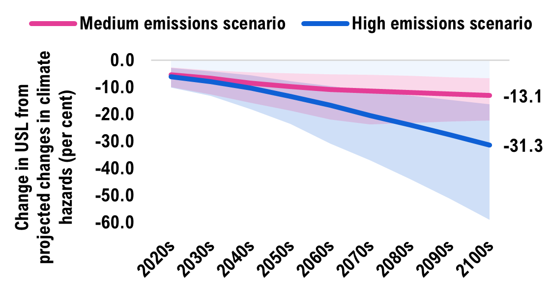
|
|
|
Operations & Maintenance 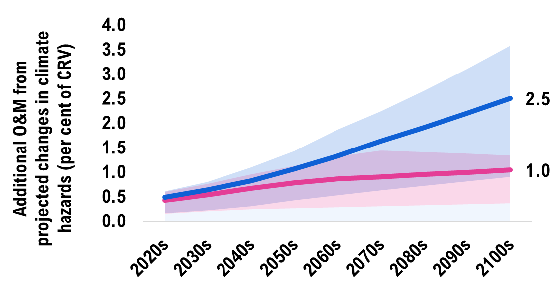
|
|
| Adaptation Costs | |
|
Retrofit Costs 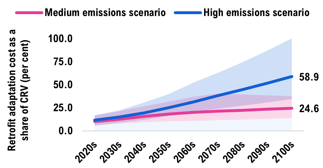
|
|
|
Renewal Costs 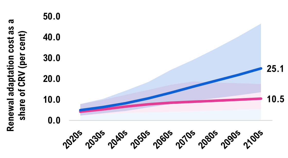
|
|
Accessible version
| In Absence of Adaptation | ||||||||||
|---|---|---|---|---|---|---|---|---|---|---|
| Useful Service Life | ||||||||||
| Emissions Scenario | 2020s | 2030s | 2040s | 2050s | 2060s | 2070s | 2080s | 2090s | 2100s | |
| Medium | Low | -2.7 | -3.7 | -4.5 | -4.8 | -5.1 | -5.4 | -5.8 | -6.2 | -6.6 |
| Median | -5.3 | -6.7 | -8.4 | -9.8 | -10.7 | -11.3 | -11.9 | -12.5 | -13.1 | |
| High | -9.8 | -12.6 | -15.7 | -18.6 | -21.8 | -23.8 | -23.2 | -22.7 | -22.2 | |
| High | Low | -2.9 | -4.1 | -5.6 | -7.6 | -9.5 | -11.4 | -13.0 | -14.6 | -16.3 |
| Median | -6.2 | -8.0 | -10.3 | -13.3 | -16.6 | -20.4 | -23.9 | -27.5 | -31.3 | |
| High | -10.0 | -13.2 | -18.1 | -23.5 | -30.8 | -37.0 | -43.9 | -51.2 | -59.0 | |
| Operations & Maintenance | ||||||||||
| Emissions Scenario | 2020s | 2030s | 2040s | 2050s | 2060s | 2070s | 2080s | 2090s | 2100s | |
| Medium | Low | 0.2 | 0.2 | 0.2 | 0.3 | 0.3 | 0.3 | 0.3 | 0.3 | 0.4 |
| Median | 0.4 | 0.5 | 0.7 | 0.8 | 0.9 | 0.9 | 1.0 | 1.0 | 1.0 | |
| High | 0.6 | 0.8 | 1.0 | 1.1 | 1.3 | 1.4 | 1.4 | 1.4 | 1.3 | |
| High | Low | 0.2 | 0.2 | 0.3 | 0.4 | 0.5 | 0.6 | 0.7 | 0.8 | 0.9 |
| Median | 0.5 | 0.6 | 0.8 | 1.1 | 1.3 | 1.6 | 1.9 | 2.2 | 2.5 | |
| High | 0.6 | 0.8 | 1.1 | 1.4 | 1.9 | 2.2 | 2.7 | 3.1 | 3.6 | |
| Adaptation Costs | ||||||||||
| Retrofit Costs | ||||||||||
| Emissions Scenario | 2020s | 2030s | 2040s | 2050s | 2060s | 2070s | 2080s | 2090s | 2100s | |
| Medium | Low | 5.8 | 7.7 | 9.4 | 10.2 | 10.8 | 11.5 | 12.3 | 13.1 | 13.9 |
| Median | 10.0 | 12.6 | 15.7 | 18.3 | 20.2 | 21.3 | 22.4 | 23.5 | 24.6 | |
| High | 16.7 | 21.3 | 26.7 | 31.6 | 37.0 | 40.3 | 39.4 | 38.5 | 37.6 | |
| High | Low | 6.1 | 8.7 | 11.8 | 16.1 | 20.1 | 24.0 | 27.4 | 30.8 | 34.4 |
| Median | 11.6 | 15.0 | 19.4 | 25.0 | 31.2 | 38.3 | 44.9 | 51.7 | 58.9 | |
| High | 17.0 | 22.4 | 30.8 | 39.9 | 52.2 | 62.9 | 74.5 | 86.9 | 100.2 | |
| Renewal Costs | ||||||||||
| Emissions Scenario | 2020s | 2030s | 2040s | 2050s | 2060s | 2070s | 2080s | 2090s | 2100s | |
| Medium | Low | 2.3 | 3.1 | 3.7 | 4.0 | 4.3 | 4.5 | 4.8 | 5.2 | 5.5 |
| Median | 4.3 | 5.4 | 6.7 | 7.8 | 8.6 | 9.1 | 9.5 | 10.0 | 10.5 | |
| High | 7.7 | 9.9 | 12.4 | 14.7 | 17.2 | 18.7 | 18.3 | 17.9 | 17.5 | |
| High | Low | 2.4 | 3.4 | 4.7 | 6.4 | 7.9 | 9.5 | 10.8 | 12.2 | 13.6 |
| Median | 4.9 | 6.4 | 8.3 | 10.6 | 13.3 | 16.3 | 19.1 | 22.0 | 25.1 | |
| High | 7.9 | 10.4 | 14.3 | 18.5 | 24.2 | 29.2 | 34.6 | 40.4 | 46.5 | |
| In Absence of Adaptation | |
|
Useful Service Life 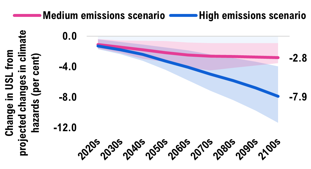
|
|
|
Operations & Maintenance 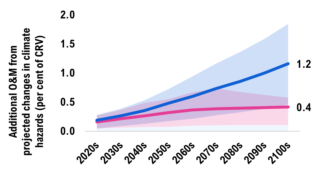
|
|
| Adaptation Costs | |
|
Retrofit Costs 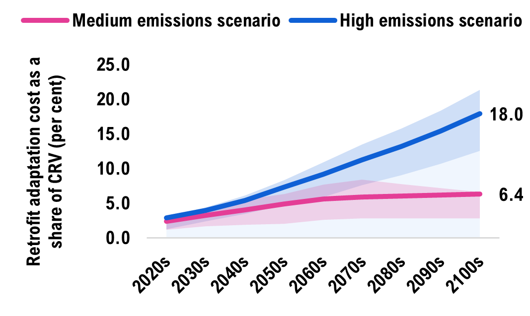
|
|
|
Renewal Costs 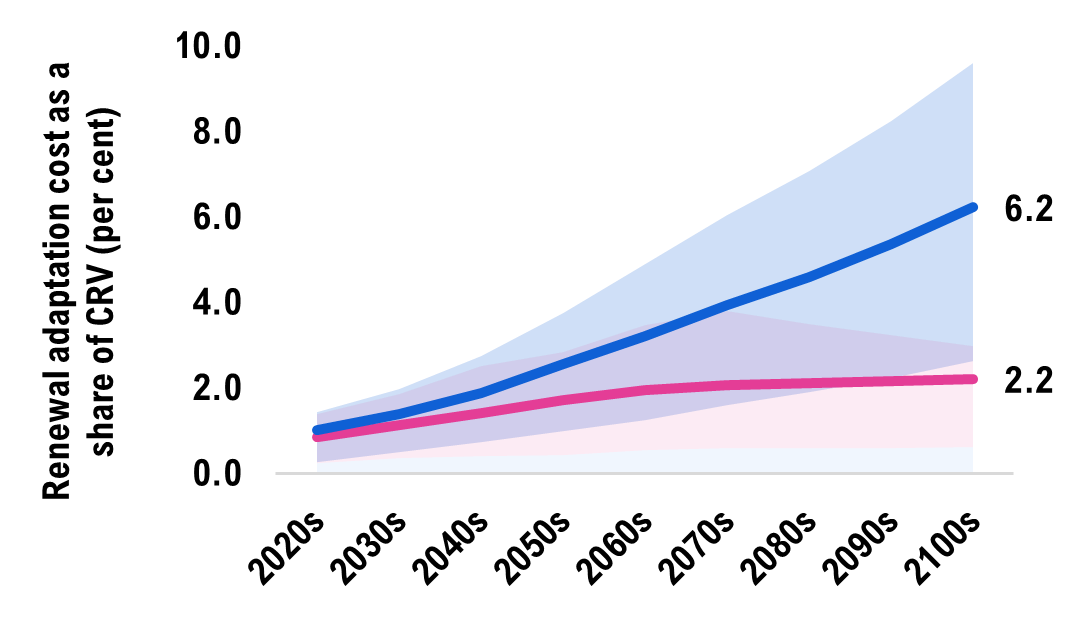
|
|
Accessible version
| In Absence of Adaptation | ||||||||||
|---|---|---|---|---|---|---|---|---|---|---|
| In Absence of Adaptation | ||||||||||
| Emissions Scenario | 2020s | 2030s | 2040s | 2050s | 2060s | 2070s | 2080s | 2090s | 2100s | |
| Medium | Low | -0.4 | -0.5 | -0.6 | -0.7 | -0.8 | -0.9 | -0.9 | -0.9 | -0.9 |
| Median | -1.1 | -1.4 | -1.8 | -2.2 | -2.5 | -2.6 | -2.7 | -2.7 | -2.8 | |
| High | -1.6 | -2.2 | -3.0 | -3.4 | -4.1 | -4.5 | -4.1 | -3.8 | -3.5 | |
| High | Low | -0.4 | -0.8 | -1.1 | -1.5 | -1.8 | -2.4 | -2.8 | -3.3 | -3.9 |
| Median | -1.3 | -1.8 | -2.4 | -3.3 | -4.1 | -5.0 | -5.8 | -6.8 | -7.9 | |
| High | -1.7 | -2.3 | -3.2 | -4.4 | -5.8 | -7.2 | -8.4 | -9.8 | -11.4 | |
| Operations & Maintenance | ||||||||||
| Emissions Scenario | 2020s | 2030s | 2040s | 2050s | 2060s | 2070s | 2080s | 2090s | 2100s | |
| Medium | Low | 0.0 | 0.1 | 0.1 | 0.1 | 0.1 | 0.1 | 0.1 | 0.1 | 0.1 |
| Median | 0.2 | 0.2 | 0.3 | 0.3 | 0.4 | 0.4 | 0.4 | 0.4 | 0.4 | |
| High | 0.3 | 0.4 | 0.5 | 0.6 | 0.7 | 0.7 | 0.7 | 0.6 | 0.6 | |
| High | Low | 0.0 | 0.1 | 0.1 | 0.2 | 0.2 | 0.3 | 0.3 | 0.4 | 0.5 |
| Median | 0.2 | 0.3 | 0.4 | 0.5 | 0.6 | 0.7 | 0.9 | 1.0 | 1.2 | |
| High | 0.3 | 0.4 | 0.5 | 0.7 | 0.9 | 1.2 | 1.4 | 1.6 | 1.8 | |
| Adaptation Costs | ||||||||||
| Retrofit Costs | ||||||||||
| Emissions Scenario | 2020s | 2030s | 2040s | 2050s | 2060s | 2070s | 2080s | 2090s | 2100s | |
| Medium | Low | 1.2 | 1.7 | 1.9 | 2.1 | 2.6 | 2.8 | 2.8 | 2.9 | 2.9 |
| Median | 2.4 | 3.3 | 4.1 | 4.9 | 5.6 | 5.9 | 6.1 | 6.2 | 6.4 | |
| High | 3.1 | 4.1 | 5.6 | 6.3 | 7.7 | 8.5 | 7.8 | 7.2 | 6.6 | |
| High | Low | 1.3 | 2.4 | 3.5 | 4.8 | 5.9 | 7.6 | 9.0 | 10.7 | 12.6 |
| Median | 2.9 | 4.0 | 5.4 | 7.4 | 9.2 | 11.3 | 13.2 | 15.4 | 18.0 | |
| High | 3.2 | 4.4 | 6.1 | 8.3 | 10.9 | 13.5 | 15.8 | 18.4 | 21.4 | |
| Renewal Costs | ||||||||||
| Emissions Scenario | 2020s | 2030s | 2040s | 2050s | 2060s | 2070s | 2080s | 2090s | 2100s | |
| Medium | Low | 0.3 | 0.4 | 0.4 | 0.4 | 0.5 | 0.6 | 0.6 | 0.6 | 0.6 |
| Median | 0.8 | 1.1 | 1.4 | 1.7 | 2.0 | 2.1 | 2.1 | 2.2 | 2.2 | |
| High | 1.4 | 1.9 | 2.5 | 2.8 | 3.5 | 3.8 | 3.5 | 3.2 | 3.0 | |
| High | Low | 0.3 | 0.5 | 0.7 | 1.0 | 1.2 | 1.6 | 1.9 | 2.2 | 2.6 |
| Median | 1.0 | 1.4 | 1.9 | 2.6 | 3.2 | 3.9 | 4.6 | 5.4 | 6.2 | |
| High | 1.4 | 2.0 | 2.7 | 3.7 | 4.9 | 6.1 | 7.1 | 8.3 | 9.6 | |
Appendix D: The contribution of individual climate hazards to key transportation infrastructure costs in the absence of adaptation
This section provides information on how the individual climate hazards deemed financially relevant by WSP contribute to infrastructure costs for asset types that are impacted by more than one climate hazard. Since only one climate hazard was assessed for both large structural culverts and transit engineering assets, climate hazard breakdowns are not presented for these asset types.
Roads
Trends in extreme rainfall and extreme heat are both projected to drive the decline in USL and increase in O&M spending of public roads in Ontario.
Figure D-1More intense rainfall and extreme heat will contribute to the decline in USL of public roads
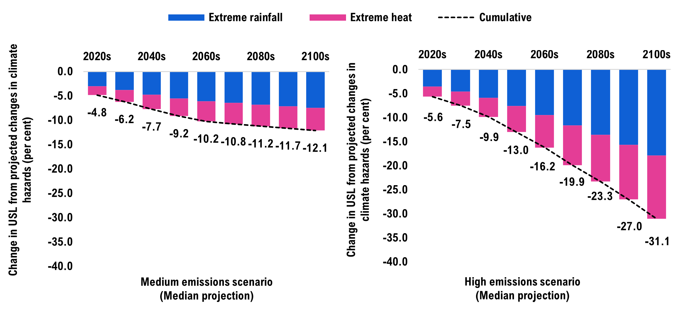
Source: FAO.
Figure D-2More intense rainfall and extreme heat will contribute to the increase in O&M of public roads
Source: FAO.
Bridges
Trends in extreme rainfall are projected to drive most of the decline in USL of public bridges in Ontario, while fewer freeze-thaw cycles will somewhat offset the negative impacts of extreme rainfall.
Figure D-3More intense rainfall will contribute the most to the decline in USL of public bridges, significantly offset by the decline in freeze-thaw cycles

Source: FAO.
Appendix E: Comparing the present value costs of different asset management strategies
As seen in Chapter 6, each asset management strategy has a different cost profile over time. The proactive adaptation strategy sees higher costs earlier in the century, while the no adaptation and reactive adaptation strategies see costs rise significantly in the latter part of the century. When evaluating alternative long-term financial decisions where the timing of costs varies, a standard approach is to discount real costs into present value dollars using a real discount rate. When discounted, costs incurred further in the future carry less weight relative to costs incurred sooner.
The appropriate discount rate for evaluating long-term financial decisions about climate change is subject to significant debate.[56] In a paper surveying over 200 experts, discount rates recommended ranged from zero to 10 per cent, with a median value of 2.3 per cent. Despite the wide range of recommended rates, over 90 per cent of respondents indicated they were comfortable with a rate between one and three per cent.[57]
Figure E-1 shows how the choice of discount rate impacts the present value of the total cost estimates for the median climate projections.
Figure E-1The present value cost of each asset management strategy under different discount rates
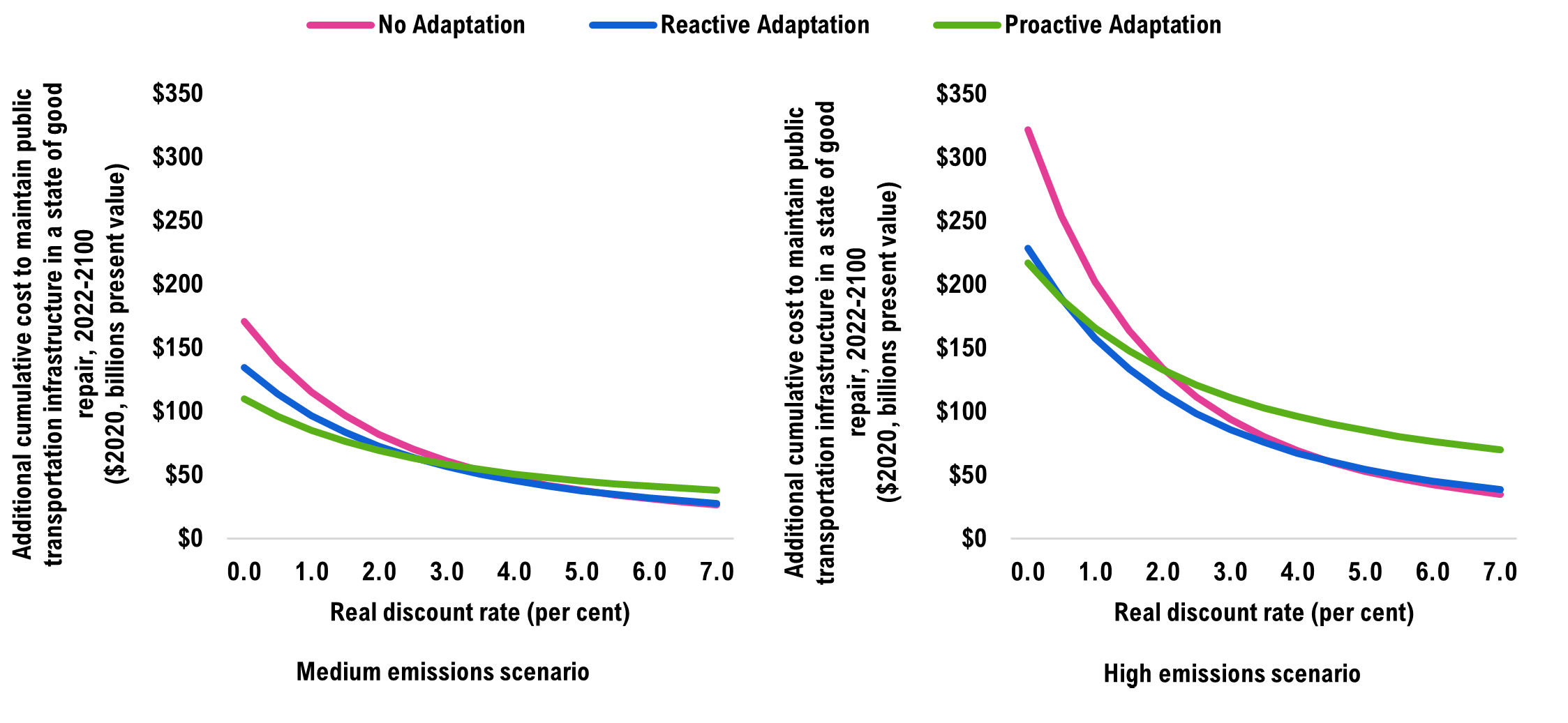
Note: The costs presented use the median (50th percentile) climate projections. Uncertainty ranges are omitted from this chart for presentation purpose.
Source: FAO.
The proactive adaptation strategy has the lowest total present value costs at discount rates approximately below 3.0 per cent (medium emissions scenario) and 1.0 per cent (high emissions scenario). The reactive adaptation strategy has the lowest present value costs at discount rates between 3.0 to 5.0 per cent (medium emissions scenario) and between 1.0 to 4.0 per cent (high emissions scenario). At higher discount rates, the present-value costs of the no adaptation strategy and the reactive adaptation strategy are essentially the same, as the cost savings from thereactive adaptationstrategy are more heavily discounted at higher rates.
However, comparing the present value costs of the different adaptation strategies as outlined above should be treated with caution. This comparison does not incorporate the costs of infrastructure service disruptions to households and businesses. For example, if a road becomes damaged and must be repaired, this analysis includes the cost of those repairs, but excludes the costs to households and businesses of traffic delays.
In addition, this comparison only includes the impacts of three climate hazards, and excludes many others (such as wildfires and permafrost degradation). Lastly, these results reflect the median projections for the medium and high emissions projections, but exclude the other possible outcomes as estimated by the climate and engineering uncertainties presented throughout the report.
Appendix F: Costing results in the low emissions scenario
While the report focused on the medium and high emissions scenario, this appendix presents the costing results of the three adaptation strategies for all emissions scenarios. The additional climate-related costs in each emissions scenario are presented as cumulative summations over the century.
In the low emissions scenario, a major and immediate turnaround in global climate policies is assumed. Emissions are projected to peak in the early 2020s and decline to zero by the 2080s, limiting the rise in global mean temperatures to 1.6°C (0.8 to 2.4°C) by 2100 compared to the pre-industrial average.[58] Even in the low emissions scenario, changes in extreme rainfall, extreme heat and freeze-thaw cycles will still have material financial impacts. Taken together, these hazards would raise the costs of maintaining Ontario’s public transportation infrastructure assets by $116 billion (11 per cent above baseline) by 2100 in the absence of adaptation.
Figure F-1The cost of maintaining the current portfolio of public transportation infrastructure will increase by $116 billion in the low emissions scenario in the absence of adaptation
Note: The solid line is the median (or 50th percentile) projection. The coloured bands represent the range of possible outcomes in each emissions scenario. The costs presented in this chart are in addition to the projected baseline costs over the same period.
Source: WSP and FAO.
Figure F-2A reactive adaptation strategy, where assets are adapted at the end of their service life to withstand the impacts of climate hazards, will add $93 billion in infrastructure costs over the century in the low emissions scenario
Note: The solid line is the median (or 50th percentile) projection. The coloured bands represent the range of possible outcomes in each emissions scenario. The costs presented in this chart are in addition to the projected baseline costs over the same period.
Source: WSP and FAO.
Figure F-3A proactive adaptation strategy, where assets are adapted at the earliest opportunity to withstand the impacts of climate hazards, will add $64 billion in infrastructure costs over the century in the low emissions scenario
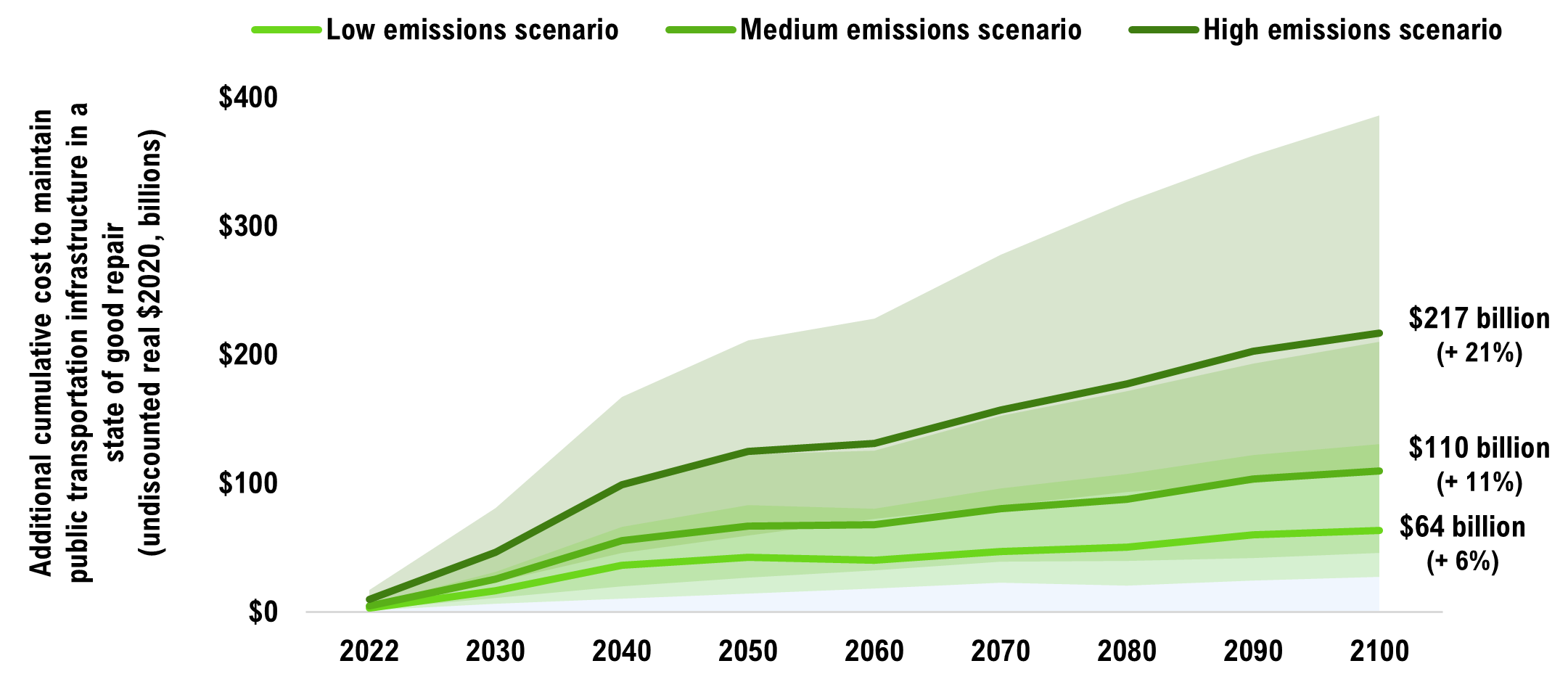
Note: The solid line is the median (or 50th percentile) projection. The coloured bands represent the range of possible outcomes in each emissions scenario. The costs presented in this chart are in addition to the projected baseline costs over the same period.
Source: WSP and FAO.
Appendix G: Breakdown of cumulative costs under different adaptation strategies by asset type
| Cumulative Additional Costs (2022-2100) | |||||
|---|---|---|---|---|---|
| Emissions Scenario | Estimate | Base | No Adaptation ($ Billions) | Reactive Adaptation ($ Billions) | Proactive Adaptation ($ Billions) |
| Medium | Low | $791 | $73 (9%) |
$58 (7%) |
$46 (6%) |
| Median | $133 (17%) |
$106 (13%) |
$96 (12%) |
||
| High | $238 (30%) |
$184 (23%) |
$177 (22%) |
||
| High | Low | $152 (19%) |
$109 (14%) |
$107 (14%) |
|
| Median | $258 (33%) |
$179 (23%) |
$191 (24%) |
||
| High | $420 (53%) |
$292 (37%) |
$331 (42%) |
||
| Cumulative Additional Costs (2022-2100) | |||||
|---|---|---|---|---|---|
| Emissions Scenario | Estimate | Base | No Adaptation ($ Billions) | Reactive Adaptation ($ Billions) | Proactive Adaptation ($ Billions) |
| Medium | Low | $110 | $8 (7%) |
$4 (4%) |
-$4 * (-4%) |
| Median | $19 (17%) |
$15 (14%) |
$5 (4%) |
||
| High | $33 (30%) |
$30 (27%) |
$18 (16%) |
||
| High | Low | $15 (13%) |
$8 (8%) |
-$6 * (-5%) |
|
| Median | $35 (31%) |
$28 (25%) |
$9 (8%) |
||
| High | $53 (48%) |
$47 (43%) |
$29 (26%) |
||
| Cumulative Additional Costs (2022-2100) | |||||
|---|---|---|---|---|---|
| Emissions Scenario | Estimate | Base | No Adaptation ($ Billions) | Reactive Adaptation ($ Billions) | Proactive Adaptation ($ Billions) |
| Medium | Low | $22 | $4 (18%) |
$4 (17%) |
$3 (14%) |
| Median | $11 (48%) |
$9 (42%) |
$6 (29%) |
||
| High | $16 (73%) |
$14 (65%) |
$10 (46%) |
||
| High | Low | $7 (34%) |
$7 (32%) |
$6 (27%) |
|
| Median | $18 (80%) |
$15 (69%) |
$11 (49%) |
||
| High | $31 (139%) |
$26 (120%) |
$17 (78%) |
||
| Cumulative Additional Costs (2022-2100) | |||||
|---|---|---|---|---|---|
| Emissions Scenario | Estimate | Base | No Adaptation ($ Billions) | Reactive Adaptation ($ Billions) | Proactive Adaptation ($ Billions) |
| Medium | Low | $92 | $4 (4%) |
$1 (1%) |
$1 (1%) |
| Median | $8 (8%) |
$5 (5%) |
$3 (3%) |
||
| High | $11 (12%) |
$7 (7%) |
$5 (5%) |
||
| High | Low | $6 (7%) |
$4 (4%) |
$4 (4%) |
|
| Median | $11 (12%) |
$7 (7%) |
$6 (7%) |
||
| High | $18 (20%) |
$9 (10%) |
$9 (10%) |
||
8 | References
Asset Management BC, Climate Change and Asset Management: A Sustainable Service Delivery Primer.
Bush, E. and Lemmen, D.S., editors, 2019, Canada in a Changing Climate: National Issues Report – Chapter 6: Costs and Benefits of Climate Change Impacts and Adaptation, Government of Canada, Ottawa, ON.
Canadian Standards Association, 2014, Canadian Highway Bridge Design Code.
Cannon, A.J., Jeong, D.I., Zhang, X., and Zwiers, F.W., 2020, Climate-Resilient Buildings and Core Public Infrastructure: An Assessment of the Impact of Climate Change on Climatic Design Data in Canada, Government of Canada.
Chinowsky, P., Helman, J., Gulati, S., Neumann, J., and Martinich, J., 2019, Impacts of climate change on operation of the US rail network. Transport Policy (75), 183-191.
Drupp, M., Freeman, M., Groom, B., and Nesje, F., 2015, Discounting disentangled: an expert survey on the determinants of the long-term social discount rate. Working Paper172. Grantham Research Institute on Climate Change and the Environment, London School of Economics and Political Science, London, United Kingdom.
Federation of Canadian Municipalities, 2020, Investing in Canada’s Future: The Cost of Climate Adaptation at the Local Level.
Financial Accountability Office of Ontario, 2020, Provincial Infrastructure.
Financial Accountability Office of Ontario, 2021a, Municipal Infrastructure.
Financial Accountability Office of Ontario, 2021b, Costing Climate Change Impacts to Public Infrastructure: Project Backgrounder and Methodology.
Financial Accountability Office of Ontario, 2021c, Costing Climate Change Impacts to Public Infrastructure: Assessing the financial impacts of extreme rainfall, extreme heat and freeze-thaw cycles on public buildings in Ontario.
Government of Canada, 2019, Infrastructure Canada’s Climate Lens.
Government of Canada, 2021, Natural Resources Canada’s Canada’s Climate Change Adaptation Platform.
Government of Canada, 2022, Infrastructure Canada’s Climate-Resilient Buildings and Core Public Infrastructure Initiative
HDR, 2008, Costs of Road Congestion in the Greater Toronto and Hamilton Area: Impact and Cost Benefit Analysis of the Metrolinx Draft Regional Transportation Plan. Report produced for Metrolinx.
Institute for Catastrophic Loss Reduction, 2020,Estimating the benefits of Climate Resilient Buildings and Core Public Infrastructure (CRBCPI).
Intergovernmental Panel on Climate Change, 2013, Climate Change 2013: The Physical Science Basis: Annex II: Climate System Scenario Tables.
Intergovernmental Panel on Climate Change, 2014, Climate Change 2014: Impacts, Adaptation, and Vulnerability, Chapter 17: Economics of Adaptation.
Intergovernmental Panel on Climate Change, 2014, AR5 Synthesis Report: Climate Change 2014.
Intergovernmental Panel on Climate Change, 2021, Climate Change 2021: The Physical Science Basis: Summary for Policymakers.
International Institute of Sustainable Development, 2021,Advancing the Climate Resilience of Canadian Infrastructure: A review of literature to inform the way forward.
Meyer, M.D., Amekudzi, A., and O’Har, J.P., 2010, Transportation asset management systems and climate change: adaptive systems management approach. Transportation Research Record, (2160), 12-20.
Ness, R., Clark, D. G., Bourque, J., Coffman, D., and Beugin, D., 2021, Under Water: The Costs of Climate Change for Canada’s Infrastructure, Canadian Climate Institute.
Neumann, J.E., Chinowsky, P., Helman, J.et al., 2021, Climate effects on US infrastructure: the economics of adaptation for rail, roads, and coastal development.Climatic Change(167),44.
Ontario Ministry of Transportation, 2017, Addressing Climate Change through Engineering Practice.
Organisation for Economic Cooperation and Development (OECD), 2018, Climate-Resilient Infrastructure.
Pacific Climate Impacts Consortium, 2021, PCIC Science Brief: Should the RCP 8.5 emissions scenario represent “business as usual?”.
Palko, K. and Lemmen, D.S., editors, 2017, Climate risks and adaptation practices for the Canadian transportation sector 2016.
Transport Canada, 2021, Projects funded by the Northern Transportation Adaptation Initiative.
United Nations Environment Program (UNEP), 2021, Buildings and Climate Change Adaptation: A Call to Action.
United Nations Framework Convention on Climate Change, 2011, Assessing the Costs and Benefits of Adaptation Options: An Overview of Approaches.
Warren, F.J. and Lemmen, D.S., editors, 2014, Canada in a Changing Climate: Sector Perspectives on Impacts and Adaptation, Government of Canada.
Warren, F.J. and Lulham, N., editors, 2021, Canada in a Changing Climate:National Issues Report, Government of Canada.
WSP, 2021, Costing climate change impacts and adaptation for provincial and municipal public infrastructure in Ontario, Deliverable #10 – Final Report, Toronto, Ontario. Report produced for Financial Accountability Office of Ontario.
- Previously Released: Reports on Ontario’s Provincial Infrastructure and Ontario’s Municipal Infrastructure, CIPI Project Backgrounder and Methodology, WSP Report, and Report on Buildings and Facilities.
- Current Report: Report on Public Transportation Infrastructure
- Upcoming in 2022: Reports on Public Water Infrastructure and Summary Report
| Medium Emissions Scenario | High Emissions Scenario | |
|---|---|---|
| No adaptation – additional climate-related costs | $171 | $322 |
| Reactive adaptation strategy – additional climate-related costs | $135 | $229 |
| Proactive adaptation strategy – additional climate-related costs | $110 | $217 |
| Level of Government | Sector | CRV | Share |
|---|---|---|---|
| Municipal | Bridges | $35 | 10% |
| Large Structural Culverts | $7 | 2% | |
| Roads | $221 | 67% | |
| Transit Engineering | $6 | 2% | |
| Provincial | Bridges | $23 | 7% |
| Large Structural Culverts | $5 | 2% | |
| Roads | $19 | 6% | |
| Transit Engineering | $13 | 4% |
| 2022-2030 | 2031-2070 | 2071-2100 | 2022-2100 | |
|---|---|---|---|---|
| Stable Climate | $ 11.0 | $ 13.4 | $ 12.6 | $ 12.9 |
| Extreme Heat | Extreme Rainfall | Freeze-thaw cycles | |
|---|---|---|---|
| Roads | Included in report | Included in report | Estimated but excluded from report |
| Bridges | Not estimated | Included in report | Included in report |
| Large Structural Culverts | Not estimated | Included in report | Not estimated |
| Transit Engineering | Included in report | Not estimated | Not estimated |
| Transportation Assets | Includes | Relevant Hazard |
|---|---|---|
| Roads | Pavement surface, pavement base and sub-base, embankments, retention systems, drainage systems, road finishing. | Extreme rainfall will increase erosion and washouts, while extreme heat will increase the risk of cracks forming through thermal weathering. |
| Bridges | Foundations, substructure, superstructure, decks, barriers and ancillary structures. | Extreme rainfall will more rapidly erode bridge foundations, embankments, and approaches, increasing deterioration and maintenance costs. Annual FTCs, which normally contribute to concrete cracking, are declining, benefitting these assets. |
| Large Structural Culverts | Channel protection, culverts, wingwalls and headwalls. | Extreme rainfall will cause erosion, wash outs and scour damages to channel protection and culverts. |
| Transit Engineering | Steel rails, tracks, rail braces, tie plates, insulated joints, crossings. | Higher temperature increases friction between train wheels and tracks, potentially resulting in the buckling of tracks. Extreme temperatures also reduce the viscosity of asphalt on which rail sits, increasing friction and erosion. |
| Extreme Heat | |||||||||
|---|---|---|---|---|---|---|---|---|---|
| Low Emissions Scenario | Medium Emissions Scenario | High Emissions Scenario | |||||||
| Year | Low | Median | High | Low | Median | High | Low | Median | High |
| 1950 | 1 | 3 | 5 | 1 | 3 | 5 | 1 | 3 | 5 |
| 1951 | 1 | 2 | 8 | 1 | 2 | 8 | 1 | 2 | 8 |
| 1952 | 1 | 3 | 6 | 1 | 3 | 6 | 1 | 3 | 6 |
| 1953 | 1 | 3 | 7 | 1 | 3 | 8 | 1 | 3 | 7 |
| 1954 | 1 | 2 | 4 | 1 | 2 | 4 | 1 | 2 | 4 |
| 1955 | 1 | 2 | 7 | 1 | 2 | 7 | 1 | 2 | 7 |
| 1956 | 0 | 3 | 7 | 0 | 3 | 7 | 0 | 3 | 7 |
| 1957 | 0 | 3 | 7 | 0 | 4 | 7 | 0 | 3 | 7 |
| 1958 | 1 | 2 | 4 | 1 | 2 | 4 | 1 | 2 | 4 |
| 1959 | 1 | 2 | 6 | 1 | 2 | 6 | 1 | 2 | 6 |
| 1960 | 1 | 3 | 7 | 1 | 3 | 6 | 1 | 3 | 7 |
| 1961 | 1 | 3 | 5 | 1 | 3 | 5 | 1 | 3 | 5 |
| 1962 | 0 | 2 | 5 | 0 | 2 | 5 | 0 | 2 | 5 |
| 1963 | 0 | 2 | 6 | 0 | 2 | 6 | 0 | 2 | 6 |
| 1964 | 0 | 2 | 4 | 0 | 2 | 4 | 0 | 2 | 4 |
| 1965 | 1 | 2 | 4 | 1 | 2 | 4 | 1 | 2 | 4 |
| 1966 | 0 | 2 | 5 | 0 | 2 | 5 | 0 | 2 | 5 |
| 1967 | 1 | 2 | 7 | 1 | 2 | 7 | 1 | 2 | 7 |
| 1968 | 1 | 2 | 5 | 1 | 3 | 5 | 1 | 2 | 5 |
| 1969 | 0 | 1 | 4 | 0 | 2 | 4 | 0 | 1 | 4 |
| 1970 | 1 | 3 | 7 | 1 | 2 | 6 | 1 | 3 | 7 |
| 1971 | 1 | 2 | 5 | 1 | 2 | 5 | 1 | 2 | 5 |
| 1972 | 1 | 2 | 5 | 1 | 2 | 5 | 1 | 2 | 5 |
| 1973 | 0 | 1 | 6 | 0 | 1 | 6 | 0 | 1 | 6 |
| 1974 | 1 | 2 | 5 | 1 | 3 | 5 | 1 | 2 | 5 |
| 1975 | 1 | 2 | 4 | 1 | 2 | 4 | 1 | 2 | 4 |
| 1976 | 1 | 2 | 8 | 1 | 2 | 8 | 1 | 2 | 8 |
| 1977 | 1 | 2 | 6 | 1 | 2 | 6 | 1 | 2 | 6 |
| 1978 | 1 | 2 | 5 | 1 | 2 | 5 | 1 | 2 | 5 |
| 1979 | 1 | 3 | 5 | 1 | 3 | 5 | 1 | 3 | 5 |
| 1980 | 1 | 2 | 8 | 1 | 2 | 7 | 1 | 2 | 8 |
| 1981 | 1 | 4 | 8 | 1 | 4 | 8 | 1 | 4 | 8 |
| 1982 | 1 | 3 | 7 | 1 | 3 | 7 | 1 | 3 | 7 |
| 1983 | 1 | 2 | 5 | 1 | 2 | 5 | 1 | 2 | 5 |
| 1984 | 1 | 3 | 7 | 1 | 3 | 6 | 1 | 3 | 7 |
| 1985 | 1 | 3 | 8 | 1 | 3 | 8 | 1 | 3 | 8 |
| 1986 | 1 | 4 | 6 | 1 | 3 | 6 | 1 | 4 | 6 |
| 1987 | 1 | 2 | 7 | 1 | 2 | 7 | 1 | 2 | 7 |
| 1988 | 1 | 3 | 9 | 1 | 2 | 9 | 1 | 3 | 9 |
| 1989 | 2 | 6 | 10 | 2 | 6 | 10 | 2 | 6 | 10 |
| 1990 | 1 | 3 | 8 | 1 | 3 | 8 | 1 | 3 | 8 |
| 1991 | 1 | 4 | 6 | 2 | 4 | 7 | 1 | 4 | 7 |
| 1992 | 0 | 2 | 6 | 0 | 2 | 6 | 0 | 2 | 6 |
| 1993 | 1 | 2 | 6 | 1 | 2 | 6 | 1 | 2 | 6 |
| 1994 | 2 | 4 | 6 | 2 | 4 | 6 | 2 | 4 | 6 |
| 1995 | 1 | 3 | 6 | 1 | 3 | 6 | 1 | 3 | 6 |
| 1996 | 1 | 4 | 8 | 1 | 4 | 8 | 1 | 4 | 8 |
| 1997 | 2 | 3 | 7 | 2 | 4 | 9 | 2 | 3 | 7 |
| 1998 | 2 | 4 | 6 | 2 | 4 | 6 | 1 | 4 | 6 |
| 1999 | 2 | 4 | 7 | 2 | 4 | 7 | 2 | 4 | 7 |
| 2000 | 2 | 5 | 8 | 2 | 4 | 8 | 2 | 5 | 8 |
| 2001 | 2 | 4 | 7 | 2 | 4 | 7 | 2 | 4 | 7 |
| 2002 | 2 | 5 | 9 | 2 | 4 | 9 | 2 | 5 | 9 |
| 2003 | 2 | 4 | 6 | 2 | 4 | 6 | 2 | 5 | 6 |
| 2004 | 3 | 5 | 8 | 2 | 5 | 8 | 2 | 5 | 8 |
| 2005 | 2 | 5 | 10 | 2 | 5 | 10 | 2 | 5 | 10 |
| 2006 | 2 | 4 | 12 | 2 | 4 | 9 | 2 | 5 | 13 |
| 2007 | 1 | 5 | 8 | 2 | 5 | 10 | 1 | 4 | 6 |
| 2008 | 2 | 6 | 9 | 3 | 5 | 8 | 1 | 4 | 9 |
| 2009 | 3 | 6 | 10 | 1 | 5 | 11 | 3 | 5 | 9 |
| 2010 | 2 | 4 | 10 | 3 | 5 | 9 | 3 | 5 | 9 |
| 2011 | 3 | 5 | 9 | 3 | 6 | 12 | 2 | 5 | 9 |
| 2012 | 2 | 7 | 13 | 3 | 7 | 13 | 2 | 7 | 11 |
| 2013 | 2 | 6 | 12 | 2 | 6 | 11 | 2 | 5 | 9 |
| 2014 | 2 | 5 | 17 | 3 | 5 | 13 | 3 | 8 | 15 |
| 2015 | 2 | 5 | 11 | 3 | 7 | 20 | 3 | 6 | 11 |
| 2016 | 2 | 7 | 15 | 2 | 5 | 8 | 3 | 7 | 10 |
| 2017 | 4 | 8 | 13 | 3 | 5 | 13 | 2 | 7 | 15 |
| 2018 | 2 | 6 | 16 | 2 | 5 | 16 | 3 | 8 | 13 |
| 2019 | 3 | 5 | 13 | 2 | 7 | 12 | 4 | 9 | 15 |
| 2020 | 2 | 6 | 10 | 3 | 6 | 11 | 2 | 7 | 12 |
| 2021 | 4 | 7 | 14 | 2 | 9 | 17 | 2 | 5 | 14 |
| 2022 | 2 | 7 | 15 | 3 | 8 | 12 | 3 | 8 | 19 |
| 2023 | 3 | 8 | 12 | 3 | 6 | 11 | 3 | 9 | 16 |
| 2024 | 3 | 8 | 18 | 3 | 7 | 15 | 4 | 10 | 16 |
| 2025 | 3 | 7 | 13 | 3 | 9 | 12 | 3 | 8 | 15 |
| 2026 | 4 | 7 | 15 | 3 | 8 | 14 | 2 | 8 | 16 |
| 2027 | 4 | 8 | 17 | 4 | 9 | 14 | 2 | 9 | 18 |
| 2028 | 3 | 7 | 16 | 3 | 8 | 14 | 4 | 10 | 14 |
| 2029 | 4 | 7 | 14 | 4 | 8 | 16 | 3 | 8 | 17 |
| 2030 | 4 | 8 | 12 | 2 | 9 | 18 | 6 | 10 | 14 |
| 2031 | 4 | 8 | 17 | 4 | 8 | 18 | 4 | 11 | 23 |
| 2032 | 4 | 9 | 16 | 2 | 11 | 16 | 4 | 9 | 16 |
| 2033 | 3 | 8 | 20 | 4 | 10 | 22 | 4 | 11 | 19 |
| 2034 | 5 | 11 | 18 | 3 | 12 | 16 | 4 | 10 | 21 |
| 2035 | 5 | 9 | 16 | 7 | 12 | 18 | 4 | 12 | 18 |
| 2036 | 2 | 9 | 15 | 3 | 9 | 14 | 6 | 11 | 21 |
| 2037 | 4 | 8 | 15 | 2 | 9 | 16 | 5 | 10 | 22 |
| 2038 | 5 | 10 | 17 | 6 | 11 | 20 | 7 | 17 | 23 |
| 2039 | 4 | 9 | 18 | 3 | 9 | 17 | 5 | 11 | 17 |
| 2040 | 3 | 8 | 14 | 4 | 7 | 19 | 4 | 11 | 19 |
| 2041 | 4 | 9 | 19 | 6 | 11 | 20 | 8 | 13 | 24 |
| 2042 | 5 | 10 | 17 | 5 | 13 | 20 | 4 | 11 | 20 |
| 2043 | 4 | 7 | 15 | 4 | 11 | 18 | 6 | 12 | 26 |
| 2044 | 3 | 8 | 18 | 3 | 10 | 18 | 5 | 11 | 18 |
| 2045 | 4 | 7 | 18 | 4 | 12 | 22 | 6 | 12 | 21 |
| 2046 | 4 | 8 | 18 | 5 | 11 | 20 | 5 | 14 | 22 |
| 2047 | 3 | 8 | 20 | 4 | 12 | 22 | 10 | 16 | 24 |
| 2048 | 4 | 11 | 17 | 7 | 14 | 21 | 7 | 16 | 24 |
| 2049 | 2 | 9 | 17 | 4 | 10 | 21 | 8 | 15 | 24 |
| 2050 | 4 | 9 | 20 | 4 | 12 | 21 | 8 | 15 | 30 |
| 2051 | 3 | 10 | 20 | 5 | 13 | 26 | 7 | 17 | 29 |
| 2052 | 5 | 9 | 14 | 6 | 11 | 23 | 8 | 16 | 25 |
| 2053 | 5 | 10 | 18 | 5 | 13 | 24 | 8 | 21 | 32 |
| 2054 | 2 | 8 | 20 | 6 | 11 | 21 | 10 | 17 | 28 |
| 2055 | 3 | 10 | 17 | 3 | 12 | 21 | 6 | 18 | 28 |
| 2056 | 4 | 9 | 23 | 5 | 12 | 22 | 8 | 18 | 26 |
| 2057 | 3 | 8 | 16 | 3 | 12 | 19 | 7 | 21 | 31 |
| 2058 | 4 | 10 | 16 | 4 | 13 | 28 | 12 | 22 | 33 |
| 2059 | 4 | 9 | 19 | 6 | 13 | 27 | 10 | 23 | 29 |
| 2060 | 3 | 11 | 20 | 7 | 15 | 21 | 7 | 18 | 36 |
| 2061 | 4 | 10 | 14 | 6 | 15 | 22 | 12 | 20 | 37 |
| 2062 | 4 | 10 | 21 | 8 | 13 | 24 | 8 | 24 | 32 |
| 2063 | 3 | 8 | 18 | 8 | 16 | 23 | 12 | 25 | 35 |
| 2064 | 5 | 9 | 19 | 6 | 16 | 29 | 13 | 23 | 40 |
| 2065 | 3 | 11 | 18 | 7 | 16 | 26 | 17 | 30 | 37 |
| 2066 | 4 | 9 | 19 | 5 | 12 | 25 | 10 | 27 | 45 |
| 2067 | 3 | 9 | 19 | 7 | 15 | 26 | 17 | 33 | 40 |
| 2068 | 5 | 10 | 20 | 7 | 17 | 31 | 14 | 27 | 45 |
| 2069 | 2 | 10 | 16 | 8 | 17 | 27 | 14 | 29 | 39 |
| 2070 | 3 | 9 | 16 | 8 | 16 | 25 | 12 | 23 | 35 |
| 2071 | 3 | 8 | 19 | 9 | 16 | 24 | 14 | 27 | 43 |
| 2072 | 3 | 9 | 14 | 6 | 15 | 25 | 14 | 29 | 48 |
| 2073 | 4 | 12 | 19 | 9 | 15 | 32 | 12 | 28 | 49 |
| 2074 | 5 | 7 | 15 | 7 | 14 | 34 | 12 | 30 | 49 |
| 2075 | 2 | 9 | 18 | 4 | 20 | 31 | 16 | 29 | 48 |
| 2076 | 4 | 11 | 20 | 7 | 18 | 25 | 19 | 27 | 44 |
| 2077 | 3 | 10 | 15 | 4 | 16 | 26 | 15 | 31 | 50 |
| 2078 | 3 | 8 | 18 | 7 | 18 | 33 | 19 | 34 | 51 |
| 2079 | 4 | 11 | 21 | 5 | 18 | 34 | 18 | 31 | 48 |
| 2080 | 4 | 8 | 19 | 6 | 18 | 27 | 12 | 37 | 47 |
| 2081 | 4 | 10 | 16 | 6 | 17 | 25 | 23 | 33 | 48 |
| 2082 | 4 | 9 | 14 | 9 | 17 | 34 | 20 | 37 | 55 |
| 2083 | 5 | 8 | 18 | 7 | 16 | 29 | 16 | 33 | 53 |
| 2084 | 3 | 9 | 17 | 8 | 17 | 27 | 17 | 31 | 46 |
| 2085 | 3 | 7 | 15 | 9 | 18 | 35 | 22 | 38 | 55 |
| 2086 | 5 | 11 | 21 | 9 | 17 | 25 | 17 | 36 | 57 |
| 2087 | 3 | 9 | 21 | 7 | 16 | 31 | 13 | 41 | 59 |
| 2088 | 5 | 8 | 16 | 6 | 14 | 28 | 22 | 39 | 57 |
| 2089 | 3 | 8 | 23 | 8 | 16 | 34 | 18 | 42 | 60 |
| 2090 | 4 | 9 | 19 | 8 | 16 | 33 | 20 | 41 | 61 |
| 2091 | 3 | 9 | 18 | 10 | 16 | 30 | 21 | 41 | 61 |
| 2092 | 3 | 8 | 15 | 6 | 16 | 32 | 23 | 45 | 62 |
| 2093 | 5 | 8 | 19 | 9 | 17 | 37 | 25 | 48 | 66 |
| 2094 | 3 | 7 | 18 | 8 | 18 | 37 | 22 | 41 | 65 |
| 2095 | 4 | 8 | 14 | 7 | 18 | 37 | 24 | 47 | 60 |
| 2096 | 4 | 9 | 17 | 7 | 17 | 35 | 19 | 42 | 65 |
| 2097 | 3 | 8 | 21 | 9 | 16 | 26 | 17 | 44 | 72 |
| 2098 | 5 | 11 | 18 | 7 | 16 | 30 | 21 | 46 | 66 |
| 2099 | 4 | 9 | 14 | 7 | 17 | 35 | 20 | 46 | 70 |
| 2100 | 4 | 7 | 13 | 5 | 16 | 29 | 24 | 46 | 71 |
| Extreme Rainfall | |||||||||
| Low Emissions Scenario | Medium emissions scenario | High emissions scenario | |||||||
| Year | Low | Median | High | Low | Median | High | Low | Median | High |
| 2010 | 109 | 111 | 114 | 109 | 111 | 113 | 109 | 112 | 113 |
| 2020 | 111 | 113 | 118 | 111 | 115 | 119 | 111 | 116 | 121 |
| 2030 | 113 | 115 | 121 | 114 | 118 | 124 | 114 | 121 | 126 |
| 2040 | 112 | 118 | 124 | 116 | 120 | 129 | 119 | 126 | 134 |
| 2050 | 113 | 118 | 128 | 118 | 124 | 135 | 125 | 134 | 144 |
| 2060 | 113 | 119 | 129 | 119 | 126 | 140 | 131 | 142 | 158 |
| 2070 | 114 | 118 | 128 | 119 | 128 | 144 | 137 | 150 | 170 |
| 2080 | 113 | 118 | 127 | 120 | 129 | 144 | 142 | 158 | 184 |
| Freeze-Thaw Cycles | |||||||||
| Low Emissions Scenario | Medium Emissions Scenario | High Emissions Scenario | |||||||
| Year | Low | Median | High | Low | Median | High | Low | Median | High |
| 1950 | 68 | 80 | 92 | 68 | 80 | 93 | 68 | 80 | 93 |
| 1951 | 66 | 80 | 91 | 66 | 80 | 91 | 66 | 80 | 91 |
| 1952 | 66 | 78 | 89 | 66 | 78 | 89 | 66 | 78 | 89 |
| 1953 | 64 | 78 | 87 | 64 | 78 | 87 | 64 | 78 | 87 |
| 1954 | 68 | 81 | 89 | 68 | 81 | 89 | 68 | 82 | 89 |
| 1955 | 69 | 76 | 91 | 68 | 76 | 91 | 68 | 76 | 91 |
| 1956 | 66 | 78 | 87 | 67 | 76 | 87 | 67 | 76 | 87 |
| 1957 | 66 | 80 | 91 | 66 | 80 | 91 | 66 | 80 | 91 |
| 1958 | 63 | 76 | 92 | 63 | 77 | 92 | 63 | 77 | 92 |
| 1959 | 69 | 82 | 92 | 69 | 81 | 92 | 69 | 81 | 92 |
| 1960 | 67 | 80 | 90 | 67 | 80 | 90 | 67 | 80 | 90 |
| 1961 | 64 | 77 | 92 | 65 | 77 | 92 | 65 | 77 | 92 |
| 1962 | 65 | 78 | 94 | 65 | 79 | 94 | 66 | 79 | 94 |
| 1963 | 68 | 82 | 98 | 68 | 82 | 98 | 68 | 82 | 98 |
| 1964 | 70 | 82 | 95 | 70 | 81 | 95 | 70 | 81 | 95 |
| 1965 | 67 | 76 | 90 | 67 | 76 | 90 | 67 | 75 | 90 |
| 1966 | 64 | 81 | 96 | 64 | 81 | 96 | 64 | 81 | 95 |
| 1967 | 69 | 81 | 98 | 69 | 81 | 98 | 69 | 81 | 98 |
| 1968 | 64 | 77 | 93 | 64 | 77 | 93 | 64 | 77 | 93 |
| 1969 | 67 | 78 | 92 | 67 | 78 | 93 | 67 | 78 | 92 |
| 1970 | 67 | 80 | 100 | 67 | 80 | 100 | 67 | 80 | 100 |
| 1971 | 71 | 79 | 91 | 71 | 79 | 92 | 71 | 79 | 92 |
| 1972 | 69 | 82 | 95 | 70 | 83 | 95 | 70 | 83 | 95 |
| 1973 | 67 | 79 | 90 | 67 | 79 | 90 | 67 | 79 | 90 |
| 1974 | 66 | 77 | 92 | 64 | 76 | 91 | 63 | 76 | 91 |
| 1975 | 67 | 77 | 90 | 67 | 77 | 90 | 67 | 77 | 90 |
| 1976 | 63 | 77 | 92 | 63 | 77 | 91 | 63 | 77 | 91 |
| 1977 | 71 | 84 | 94 | 72 | 84 | 94 | 71 | 84 | 94 |
| 1978 | 70 | 77 | 87 | 70 | 78 | 87 | 70 | 78 | 87 |
| 1979 | 69 | 82 | 91 | 69 | 81 | 91 | 69 | 81 | 91 |
| 1980 | 68 | 75 | 87 | 69 | 75 | 87 | 69 | 76 | 86 |
| 1981 | 66 | 78 | 88 | 66 | 78 | 88 | 66 | 78 | 88 |
| 1982 | 64 | 76 | 90 | 64 | 77 | 90 | 64 | 76 | 89 |
| 1983 | 60 | 77 | 92 | 60 | 77 | 94 | 60 | 76 | 94 |
| 1984 | 64 | 80 | 87 | 64 | 79 | 87 | 64 | 80 | 87 |
| 1985 | 57 | 73 | 85 | 57 | 73 | 85 | 57 | 72 | 85 |
| 1986 | 64 | 77 | 88 | 64 | 77 | 88 | 64 | 77 | 88 |
| 1987 | 65 | 77 | 88 | 64 | 77 | 88 | 64 | 76 | 88 |
| 1988 | 62 | 75 | 86 | 62 | 75 | 85 | 62 | 75 | 85 |
| 1989 | 61 | 77 | 89 | 61 | 77 | 89 | 61 | 77 | 89 |
| 1990 | 65 | 76 | 91 | 65 | 76 | 91 | 65 | 76 | 91 |
| 1991 | 65 | 75 | 88 | 65 | 76 | 88 | 65 | 75 | 88 |
| 1992 | 66 | 75 | 90 | 66 | 74 | 90 | 65 | 75 | 90 |
| 1993 | 68 | 77 | 93 | 68 | 78 | 95 | 69 | 78 | 95 |
| 1994 | 63 | 77 | 86 | 63 | 78 | 88 | 63 | 77 | 88 |
| 1995 | 66 | 76 | 92 | 66 | 76 | 91 | 66 | 75 | 92 |
| 1996 | 67 | 76 | 89 | 68 | 76 | 89 | 68 | 76 | 89 |
| 1997 | 63 | 78 | 90 | 63 | 77 | 90 | 63 | 77 | 90 |
| 1998 | 65 | 74 | 89 | 65 | 74 | 89 | 65 | 74 | 89 |
| 1999 | 64 | 79 | 90 | 64 | 79 | 90 | 64 | 79 | 89 |
| 2000 | 63 | 77 | 86 | 64 | 77 | 89 | 64 | 77 | 89 |
| 2001 | 66 | 75 | 84 | 66 | 75 | 84 | 66 | 75 | 84 |
| 2002 | 68 | 79 | 91 | 67 | 79 | 91 | 66 | 79 | 91 |
| 2003 | 58 | 75 | 84 | 59 | 75 | 87 | 59 | 75 | 86 |
| 2004 | 63 | 74 | 89 | 63 | 74 | 88 | 63 | 74 | 88 |
| 2005 | 65 | 79 | 95 | 65 | 78 | 91 | 66 | 78 | 91 |
| 2006 | 61 | 71 | 83 | 62 | 76 | 93 | 64 | 75 | 91 |
| 2007 | 64 | 79 | 92 | 64 | 78 | 90 | 63 | 75 | 87 |
| 2008 | 63 | 76 | 85 | 61 | 77 | 86 | 63 | 77 | 92 |
| 2009 | 65 | 78 | 92 | 63 | 78 | 93 | 64 | 77 | 90 |
| 2010 | 67 | 75 | 88 | 61 | 71 | 86 | 60 | 72 | 86 |
| 2011 | 59 | 72 | 82 | 61 | 79 | 91 | 64 | 75 | 87 |
| 2012 | 62 | 76 | 88 | 63 | 75 | 91 | 59 | 74 | 89 |
| 2013 | 63 | 75 | 86 | 62 | 78 | 93 | 61 | 75 | 87 |
| 2014 | 60 | 73 | 87 | 62 | 73 | 85 | 57 | 68 | 85 |
| 2015 | 60 | 73 | 88 | 60 | 73 | 85 | 58 | 71 | 83 |
| 2016 | 61 | 71 | 90 | 61 | 72 | 82 | 58 | 73 | 87 |
| 2017 | 57 | 70 | 87 | 62 | 74 | 85 | 63 | 73 | 86 |
| 2018 | 61 | 77 | 92 | 60 | 71 | 82 | 63 | 75 | 94 |
| 2019 | 64 | 75 | 88 | 59 | 71 | 85 | 59 | 74 | 89 |
| 2020 | 63 | 72 | 84 | 59 | 73 | 85 | 58 | 70 | 88 |
| 2021 | 63 | 74 | 83 | 59 | 73 | 87 | 62 | 70 | 83 |
| 2022 | 61 | 72 | 90 | 61 | 75 | 87 | 62 | 71 | 86 |
| 2023 | 63 | 75 | 87 | 64 | 73 | 88 | 59 | 70 | 85 |
| 2024 | 57 | 71 | 84 | 62 | 75 | 88 | 57 | 72 | 88 |
| 2025 | 55 | 70 | 90 | 63 | 74 | 87 | 56 | 70 | 84 |
| 2026 | 57 | 72 | 83 | 61 | 75 | 92 | 56 | 72 | 85 |
| 2027 | 60 | 75 | 87 | 61 | 70 | 87 | 61 | 69 | 82 |
| 2028 | 60 | 75 | 88 | 62 | 72 | 89 | 59 | 69 | 85 |
| 2029 | 61 | 75 | 89 | 59 | 69 | 84 | 60 | 74 | 83 |
| 2030 | 61 | 75 | 85 | 59 | 70 | 84 | 59 | 73 | 82 |
| 2031 | 59 | 73 | 86 | 60 | 69 | 93 | 58 | 67 | 81 |
| 2032 | 60 | 74 | 84 | 60 | 72 | 84 | 56 | 70 | 87 |
| 2033 | 64 | 76 | 87 | 59 | 72 | 84 | 60 | 70 | 82 |
| 2034 | 58 | 70 | 85 | 57 | 69 | 89 | 58 | 69 | 83 |
| 2035 | 60 | 73 | 84 | 59 | 72 | 80 | 55 | 75 | 86 |
| 2036 | 60 | 72 | 86 | 61 | 74 | 89 | 59 | 71 | 84 |
| 2037 | 58 | 72 | 84 | 58 | 72 | 83 | 57 | 71 | 86 |
| 2038 | 59 | 74 | 90 | 65 | 77 | 89 | 59 | 72 | 85 |
| 2039 | 60 | 72 | 87 | 60 | 71 | 83 | 57 | 71 | 86 |
| 2040 | 62 | 73 | 91 | 57 | 69 | 87 | 56 | 65 | 89 |
| 2041 | 56 | 71 | 83 | 55 | 72 | 85 | 54 | 69 | 81 |
| 2042 | 59 | 68 | 85 | 55 | 69 | 80 | 53 | 65 | 86 |
| 2043 | 59 | 70 | 76 | 54 | 70 | 85 | 57 | 69 | 85 |
| 2044 | 53 | 72 | 84 | 58 | 71 | 87 | 58 | 70 | 81 |
| 2045 | 61 | 74 | 84 | 60 | 74 | 85 | 59 | 66 | 81 |
| 2046 | 59 | 72 | 84 | 59 | 71 | 87 | 53 | 66 | 83 |
| 2047 | 60 | 72 | 84 | 58 | 69 | 82 | 57 | 67 | 83 |
| 2048 | 56 | 72 | 93 | 59 | 69 | 81 | 52 | 67 | 79 |
| 2049 | 56 | 71 | 86 | 56 | 73 | 82 | 56 | 68 | 85 |
| 2050 | 59 | 72 | 84 | 57 | 71 | 83 | 56 | 68 | 83 |
| 2051 | 58 | 76 | 91 | 56 | 66 | 86 | 55 | 66 | 80 |
| 2052 | 59 | 70 | 89 | 56 | 70 | 86 | 56 | 66 | 83 |
| 2053 | 60 | 73 | 88 | 59 | 70 | 86 | 58 | 73 | 88 |
| 2054 | 58 | 76 | 89 | 58 | 70 | 90 | 55 | 67 | 76 |
| 2055 | 54 | 71 | 84 | 54 | 73 | 84 | 57 | 68 | 79 |
| 2056 | 61 | 75 | 83 | 54 | 72 | 86 | 54 | 70 | 86 |
| 2057 | 60 | 73 | 86 | 54 | 69 | 84 | 56 | 66 | 83 |
| 2058 | 57 | 72 | 87 | 56 | 69 | 87 | 53 | 65 | 79 |
| 2059 | 62 | 72 | 83 | 54 | 69 | 84 | 52 | 67 | 88 |
| 2060 | 60 | 74 | 86 | 53 | 69 | 84 | 52 | 68 | 83 |
| 2061 | 55 | 71 | 87 | 58 | 73 | 87 | 53 | 67 | 82 |
| 2062 | 58 | 69 | 87 | 60 | 72 | 85 | 52 | 65 | 76 |
| 2063 | 55 | 72 | 87 | 53 | 69 | 86 | 54 | 66 | 87 |
| 2064 | 54 | 72 | 89 | 55 | 74 | 88 | 54 | 66 | 86 |
| 2065 | 58 | 73 | 82 | 55 | 71 | 87 | 60 | 69 | 81 |
| 2066 | 59 | 74 | 85 | 53 | 70 | 83 | 55 | 71 | 78 |
| 2067 | 57 | 69 | 84 | 60 | 72 | 87 | 50 | 63 | 75 |
| 2068 | 60 | 75 | 87 | 58 | 73 | 89 | 52 | 70 | 85 |
| 2069 | 60 | 71 | 85 | 57 | 69 | 83 | 54 | 65 | 81 |
| 2070 | 62 | 75 | 88 | 56 | 67 | 78 | 53 | 68 | 85 |
| 2071 | 55 | 72 | 82 | 58 | 70 | 84 | 52 | 66 | 77 |
| 2072 | 57 | 72 | 86 | 53 | 68 | 81 | 53 | 66 | 79 |
| 2073 | 58 | 73 | 84 | 59 | 69 | 84 | 54 | 66 | 83 |
| 2074 | 59 | 68 | 83 | 55 | 64 | 81 | 53 | 66 | 81 |
| 2075 | 57 | 70 | 83 | 52 | 68 | 88 | 52 | 64 | 81 |
| 2076 | 59 | 70 | 83 | 53 | 69 | 88 | 53 | 67 | 83 |
| 2077 | 57 | 74 | 87 | 57 | 68 | 89 | 55 | 63 | 79 |
| 2078 | 58 | 71 | 91 | 55 | 68 | 83 | 50 | 63 | 81 |
| 2079 | 57 | 71 | 83 | 54 | 70 | 81 | 50 | 66 | 81 |
| 2080 | 56 | 74 | 88 | 50 | 66 | 83 | 56 | 66 | 82 |
| 2081 | 56 | 69 | 83 | 55 | 64 | 79 | 53 | 65 | 81 |
| 2082 | 57 | 72 | 87 | 52 | 69 | 84 | 50 | 66 | 80 |
| 2083 | 58 | 70 | 87 | 56 | 70 | 86 | 53 | 68 | 84 |
| 2084 | 58 | 70 | 88 | 57 | 74 | 96 | 52 | 65 | 86 |
| 2085 | 61 | 70 | 84 | 55 | 65 | 77 | 50 | 63 | 81 |
| 2086 | 62 | 77 | 88 | 51 | 68 | 85 | 50 | 64 | 78 |
| 2087 | 62 | 72 | 90 | 58 | 71 | 85 | 50 | 59 | 80 |
| 2088 | 55 | 71 | 90 | 58 | 70 | 82 | 48 | 66 | 90 |
| 2089 | 58 | 75 | 84 | 57 | 67 | 81 | 48 | 64 | 86 |
| 2090 | 56 | 75 | 85 | 55 | 69 | 86 | 53 | 69 | 85 |
| 2091 | 56 | 73 | 88 | 56 | 69 | 83 | 43 | 64 | 80 |
| 2092 | 62 | 75 | 88 | 57 | 72 | 86 | 56 | 67 | 81 |
| 2093 | 59 | 73 | 81 | 57 | 71 | 84 | 51 | 63 | 81 |
| 2094 | 59 | 73 | 85 | 55 | 67 | 84 | 51 | 65 | 83 |
| 2095 | 59 | 72 | 87 | 55 | 67 | 82 | 50 | 64 | 80 |
| 2096 | 54 | 68 | 86 | 57 | 70 | 85 | 54 | 65 | 81 |
| 2097 | 56 | 72 | 87 | 59 | 68 | 79 | 51 | 66 | 75 |
| 2098 | 58 | 72 | 85 | 53 | 67 | 82 | 51 | 63 | 79 |
| 2099 | 58 | 73 | 92 | 58 | 71 | 86 | 49 | 64 | 81 |
| 2100 | 60 | 76 | 89 | 48 | 67 | 87 | 48 | 63 | 81 |
| Emissions Scenario | 2022-2030 | 2031-2070 | 2071-2100 | 2022-2100 | |
|---|---|---|---|---|---|
| Medium | Stable Climate | $11.0 | $13.4 | $12.6 | $12.9 |
| No adaptation strategy, additional climate-related costs | $1.4 | $2.4 | $2.1 | $2.2 | |
| High | Stable Climate | $11.0 | $13.4 | $12.6 | $12.9 |
| No adaptation strategy, additional climate-related costs | $1.6 | $3.1 | $6.1 | $4.1 | |
| Emissions Scenario | Projection | 2022-2030 | 2031-2070 | 2070-2100 |
|---|---|---|---|---|
| Medium | Low | $0.8 | $1.0 | $1.4 |
| Median | $1.4 | $2.4 | $2.1 | |
| High | $2.1 | $3.8 | $4.2 | |
| High | Low | $0.9 | $2.1 | $3.0 |
| Median | $1.6 | $3.1 | $6.1 | |
| High | $2.3 | $5.3 | $9.7 |
| Emissions Scenario | Projection | ||
|---|---|---|---|
| Medium | Stable Climate | NA | $1,015 |
| No adaptation – additional climate-related costs | Low | $89 | |
| Median | $171 | ||
| High | $298 | ||
| High | Stable Climate | NA | $1,015 |
| No adaptation – additional climate-related costs | Low | $180 | |
| Median | $322 | ||
| High | $522 | ||
| Remaining useful life categories | Share of transportation assets by CRV (Per Cent) |
|---|---|
| Beyond useful life | 1 |
| 0-20 years | 3 |
| 20-40 years | 24 |
| 40-60 years | 57 |
| 60-80 years | 5 |
| 80-100 years | 10 |
| Transportation Assets | Adaptation |
|---|---|
| Roads | Using a higher temperature grade asphalt binder can help reduce the risk of permanent deformation from extreme heat. |
| Bridges | Deeper foundations will be less vulnerable to extreme rainfall and its anticipated effects of scour and erosion. Added rip rap for foundations in watercourses will increase erosion protection and runoff control. |
| Large Structural Culverts | Larger pipes and structures and associated excavations are needed for increased capacity in anticipation of the peak flow volume of projected extreme rainfalls. Rocks of larger diameters are required for channel protection. |
| Transit Engineering | Adequate tie plates and anchors are required to accommodate the dilatation of rail and increase stability. Increase the use of designed materials that are tolerant to higher operating temperatures in moving components and tracks. |
| Proportion of adapted public transportation by CRV (per cent) | ||
|---|---|---|
| Year | Reactive adaptation | Proactive adaptation |
| 2022 | 9 | 15 |
| 2023 | 9 | 20 |
| 2024 | 9 | 37 |
| 2025 | 9 | 39 |
| 2026 | 9 | 42 |
| 2027 | 9 | 45 |
| 2028 | 9 | 47 |
| 2029 | 9 | 48 |
| 2030 | 9 | 53 |
| 2031 | 9 | 67 |
| 2032 | 9 | 70 |
| 2033 | 10 | 71 |
| 2034 | 10 | 75 |
| 2035 | 10 | 84 |
| 2036 | 10 | 87 |
| 2037 | 10 | 87 |
| 2038 | 11 | 92 |
| 2039 | 11 | 94 |
| 2040 | 12 | 95 |
| 2041 | 13 | 96 |
| 2042 | 13 | 97 |
| 2043 | 13 | 97 |
| 2044 | 13 | 97 |
| 2045 | 14 | 99 |
| 2046 | 14 | 99 |
| 2047 | 14 | 99 |
| 2048 | 15 | 99 |
| 2049 | 18 | 99 |
| 2050 | 19 | 99 |
| 2051 | 20 | 100 |
| 2052 | 23 | 100 |
| 2053 | 25 | 100 |
| 2054 | 25 | 100 |
| 2055 | 25 | 100 |
| 2056 | 25 | 100 |
| 2057 | 26 | 100 |
| 2058 | 27 | 100 |
| 2059 | 27 | 100 |
| 2060 | 29 | 100 |
| 2061 | 39 | 100 |
| 2062 | 40 | 100 |
| 2063 | 42 | 100 |
| 2064 | 43 | 100 |
| 2065 | 46 | 100 |
| 2066 | 51 | 100 |
| 2067 | 53 | 100 |
| 2068 | 61 | 100 |
| 2069 | 64 | 100 |
| 2070 | 66 | 100 |
| 2071 | 71 | 100 |
| 2072 | 79 | 100 |
| 2073 | 81 | 100 |
| 2074 | 83 | 100 |
| 2075 | 86 | 100 |
| 2076 | 86 | 100 |
| 2077 | 86 | 100 |
| 2078 | 86 | 100 |
| 2079 | 86 | 100 |
| 2080 | 86 | 100 |
| 2081 | 87 | 100 |
| 2082 | 87 | 100 |
| 2083 | 87 | 100 |
| 2084 | 87 | 100 |
| 2085 | 87 | 100 |
| 2086 | 87 | 100 |
| 2087 | 87 | 100 |
| 2088 | 87 | 100 |
| 2089 | 87 | 100 |
| 2090 | 87 | 100 |
| 2091 | 87 | 100 |
| 2092 | 87 | 100 |
| 2093 | 88 | 100 |
| 2094 | 88 | 100 |
| 2095 | 88 | 100 |
| 2096 | 88 | 100 |
| 2097 | 88 | 100 |
| 2098 | 88 | 100 |
| 2099 | 89 | 100 |
| 2100 | 90 | 100 |
| Emissions Scenario | 2022-2030 | 2031-2070 | 2071-2100 | 2022-2100 | |
|---|---|---|---|---|---|
| Medium | Stable Climate | $ 11.0 | $ 13.4 | $ 12.6 | $ 12.9 |
| Reactive adaptation strategy, additional climate-related costs | $ 1.6 | $ 2.4 | $ 0.8 | $ 1.7 | |
| High | Stable Climate | $ 11.0 | $ 13.4 | $ 12.6 | $ 12.9 |
| Reactive adaptation strategy, additional climate-related costs | $ 2.1 | $ 3.4 | $ 2.5 | $ 2.9 | |
| Emissions Scenario | Projection | 2022-2030 | 2031-2070 | 2070-2100 |
|---|---|---|---|---|
| Medium | Low | $ 0.9 | $ 1.0 | $ 0.7 |
| Median | $ 1.6 | $ 2.4 | $ 0.8 | |
| High | $ 2.6 | $ 4.0 | $ 1.7 | |
| High | Low | $ 1.1 | $ 2.2 | $ 1.0 |
| Median | $ 2.1 | $ 3.4 | $ 2.5 | |
| High | $ 3.2 | $ 6.2 | $ 3.3 |
| Emissions Scenario | Projection | ||
|---|---|---|---|
| Medium | Stable Climate | NA | $ 1,015 |
| Reactive adaptation strategy – additional climate-related costs | Low | $ 67 | |
| Median | $ 135 | ||
| High | $ 235 | ||
| High | Stable Climate | NA | $ 1,015 |
| Reactive adaptation strategy – additional climate-related costs | Low | $ 129 | |
| Median | $ 229 | ||
| High | $ 374 | ||
| Emissions Scenario | 2022-2030 | 2031-2070 | 2071-2100 | 2022-2100 | |
|---|---|---|---|---|---|
| Medium | Stable Climate | $ 11.0 | $ 13.4 | $ 12.6 | $ 12.9 |
| Proactive adaptation strategy, additional climate-related costs | $ 2.9 | $ 1.4 | $ 1.0 | $ 1.4 | |
| High | Stable Climate | $ 11.0 | $ 13.4 | $ 12.6 | $ 12.9 |
| Proactive adaptation strategy, additional climate-related costs | $ 5.2 | $ 2.8 | $ 2.0 | $ 2.7 | |
| Emissions Scenario | Projection | 2022-2030 | 2031-2070 | 2070-2100 |
|---|---|---|---|---|
| Medium | Low | $ 1.3 | $ 0.7 | $ 0.2 |
| Median | $ 2.9 | $ 1.4 | $ 1.0 | |
| High | $ 5.1 | $ 2.7 | $ 1.9 | |
| High | Low | $ 2.6 | $ 1.5 | $ 0.9 |
| Median | $ 5.2 | $ 2.8 | $ 2.0 | |
| High | $ 9.0 | $ 4.9 | $ 3.6 |
| Emissions Scenario | Projection | ||
|---|---|---|---|
| Medium | Stable Climate | NA | $ 1,015 |
| Proactive adaptation strategy – additional climate-related costs | Low | $ 46 | |
| Median | $ 110 | ||
| High | $ 210 | ||
| High | Stable Climate | NA | $ 1,015 |
| Proactive adaptation strategy – additional climate-related costs | Low | $ 111 | |
| Median | $ 217 | ||
| High | $ 386 | ||
| Medium emissions scenario | High emissions scenario | |
|---|---|---|
| No adaptation – additional climate-related costs | $171 | $322 |
| Reactive adaptation strategy – additional climate-related costs | $135 | $229 |
| Proactive adaptation strategy – additional climate-related costs | $110 | $217 |
| Emissions Scenario | Strategy | 2022 | 2030 | 2040 | 2050 | 2060 | 2070 | 2080 | 2090 | 2100 |
|---|---|---|---|---|---|---|---|---|---|---|
| High Emissions Scenario | Reactive adaptation | $5 | $19 | $43 | $61 | $96 | $154 | $172 | $194 | $229 |
| Proactive adaptation | $10 | $47 | $99 | $125 | $131 | $157 | $177 | $203 | $217 | |
| No adaptation | $1 | $14 | $38 | $59 | $88 | $138 | $171 | $244 | $322 | |
| Medium Emissions Scenario | Reactive adaptation | $3 | $14 | $35 | $46 | $49 | $110 | $99 | $117 | $135 |
| Proactive adaptation | $5 | $26 | $56 | $67 | $68 | $80 | $88 | $103 | $110 | |
| No adaptation | $1 | $12 | $33 | $47 | $50 | $107 | $107 | $140 | $171 |
| Medium Emissions Scenario | High Emissions Scenario | |||||
|---|---|---|---|---|---|---|
| Extreme rainfall | Extreme heat | Cumulative | Extreme rainfall | Extreme heat | Cumulative | |
| 2020s | -3.0 | -1.8 | -4.8 | -3.5 | -2.1 | -5.6 |
| 2030s | -3.8 | -2.4 | -6.2 | -4.6 | -2.9 | -7.5 |
| 2040s | -4.8 | -3.0 | -7.7 | -5.9 | -4.0 | -9.9 |
| 2050s | -5.6 | -3.6 | -9.2 | -7.6 | -5.4 | -13.0 |
| 2060s | -6.1 | -4.1 | -10.2 | -9.5 | -6.8 | -16.2 |
| 2070s | -6.5 | -4.3 | -10.8 | -11.6 | -8.3 | -19.9 |
| 2080s | -6.8 | -4.4 | -11.2 | -13.6 | -9.7 | -23.3 |
| 2090s | -7.1 | -4.6 | -11.7 | -15.7 | -11.3 | -27.0 |
| 2100s | -7.5 | -4.7 | -12.1 | -17.9 | -13.2 | -31.1 |
| Medium Emissions Scenario | High Emissions Scenario | |||||
|---|---|---|---|---|---|---|
| Extreme rainfall | Extreme heat | Cumulative | Extreme rainfall | Extreme heat | Cumulative | |
| 2020s | 0.1 | 0.1 | 0.2 | 0.2 | 0.1 | 0.3 |
| 2030s | 0.2 | 0.1 | 0.3 | 0.2 | 0.1 | 0.4 |
| 2040s | 0.2 | 0.1 | 0.4 | 0.3 | 0.2 | 0.5 |
| 2050s | 0.3 | 0.2 | 0.4 | 0.3 | 0.3 | 0.6 |
| 2060s | 0.3 | 0.2 | 0.5 | 0.4 | 0.3 | 0.8 |
| 2070s | 0.3 | 0.2 | 0.5 | 0.5 | 0.4 | 0.9 |
| 2080s | 0.3 | 0.2 | 0.5 | 0.6 | 0.5 | 1.1 |
| 2090s | 0.3 | 0.2 | 0.5 | 0.7 | 0.5 | 1.3 |
| 2100s | 0.3 | 0.2 | 0.6 | 0.8 | 0.6 | 1.5 |
| Medium Emissions Scenario | High Emissions Scenario | |||||
|---|---|---|---|---|---|---|
| Extreme rainfall | Extreme heat | Cumulative | Extreme rainfall | Extreme heat | Cumulative | |
| 2020s | -1.5 | 0.8 | -0.7 | -1.7 | 1.0 | -0.7 |
| 2030s | -1.9 | 1.2 | -0.7 | -2.2 | 1.5 | -0.7 |
| 2040s | -2.3 | 1.6 | -0.8 | -2.9 | 2.0 | -0.9 |
| 2050s | -2.7 | 1.8 | -0.9 | -3.7 | 2.7 | -1.0 |
| 2060s | -3.0 | 2.1 | -0.9 | -4.6 | 3.5 | -1.1 |
| 2070s | -3.2 | 2.4 | -0.8 | -5.7 | 4.3 | -1.4 |
| 2080s | -3.3 | 2.6 | -0.7 | -6.7 | 5.0 | -1.7 |
| 2090s | -3.5 | 2.9 | -0.6 | -7.7 | 5.6 | -2.1 |
| 2100s | -3.7 | 3.1 | -0.6 | -8.8 | 6.2 | -2.6 |
| Interest Rate | Medium Emissions Scenario | High Emissions Scenario | ||||
|---|---|---|---|---|---|---|
| No adaptation | Reactive adaptation | Proactive adaptation | No adaptation | Reactive adaptation | Proactive adaptation | |
| 0.0% | $171 | $135 | $110 | $322 | $229 | $217 |
| 0.5% | $139 | $113 | $96 | $253 | $189 | $188 |
| 1.0% | $115 | $97 | $85 | $202 | $158 | $166 |
| 1.5% | $96 | $83 | $76 | $164 | $133 | $148 |
| 2.0% | $82 | $72 | $69 | $134 | $114 | $133 |
| 2.5% | $70 | $64 | $63 | $112 | $99 | $121 |
| 3.0% | $61 | $56 | $58 | $94 | $86 | $111 |
| 3.5% | $53 | $50 | $54 | $80 | $76 | $103 |
| 4.0% | $47 | $45 | $51 | $69 | $67 | $96 |
| 4.5% | $42 | $41 | $48 | $60 | $60 | $90 |
| 5.0% | $38 | $38 | $45 | $53 | $54 | $85 |
| 5.5% | $34 | $34 | $43 | $47 | $50 | $81 |
| 6.0% | $31 | $32 | $41 | $42 | $45 | $77 |
| 6.5% | $29 | $30 | $39 | $38 | $42 | $73 |
| 7.0% | $27 | $28 | $38 | $35 | $39 | $70 |
| Emissions Scenario | 2022 | 2030 | 2040 | 2050 | 2060 | 2070 | 2080 | 2090 | 2100 | |
|---|---|---|---|---|---|---|---|---|---|---|
| Low | Low | $0 | $6 | $14 | $9 | $16 | $25 | $31 | $39 | $45 |
| Median | $1 | $12 | $30 | $40 | $38 | $79 | $74 | $91 | $116 | |
| High | $1 | $17 | $44 | $63 | $68 | $135 | $133 | $165 | $193 | |
| Medium | Low | $0 | $7 | $18 | $21 | $23 | $48 | $49 | $69 | $89 |
| Median | $1 | $12 | $33 | $47 | $50 | $107 | $107 | $140 | $171 | |
| High | $1 | $19 | $49 | $80 | $119 | $173 | $191 | $253 | $298 | |
| High | Low | $0 | $8 | $20 | $35 | $36 | $91 | $86 | $135 | $180 |
| Median | $1 | $14 | $38 | $59 | $88 | $138 | $171 | $244 | $322 | |
| High | $1 | $21 | $51 | $90 | $143 | $232 | $268 | $390 | $522 | |
| Emissions Scenario | 2022 | 2030 | 2040 | 2050 | 2060 | 2070 | 2080 | 2090 | 2100 | |
|---|---|---|---|---|---|---|---|---|---|---|
| Low | Low | $1 | $7 | $14 | $9 | $14 | $24 | $31 | $36 | $38 |
| Median | $2 | $12 | $30 | $37 | $36 | $77 | $70 | $76 | $93 | |
| High | $3 | $19 | $46 | $61 | $67 | $140 | $124 | $145 | $169 | |
| Medium | Low | $1 | $8 | $19 | $18 | $22 | $46 | $47 | $50 | $67 |
| Median | $3 | $14 | $35 | $46 | $49 | $110 | $99 | $117 | $135 | |
| High | $5 | $23 | $53 | $79 | $125 | $185 | $185 | $208 | $235 | |
| High | Low | $3 | $10 | $22 | $35 | $38 | $98 | $84 | $101 | $129 |
| Median | $5 | $19 | $43 | $61 | $96 | $154 | $172 | $194 | $229 | |
| High | $9 | $29 | $61 | $98 | $163 | $276 | $263 | $314 | $374 | |
| Emissions Scenario | 2022 | 2030 | 2040 | 2050 | 2060 | 2070 | 2080 | 2090 | 2100 | |
|---|---|---|---|---|---|---|---|---|---|---|
| Low | Low | $1 | $7 | $10 | $15 | $18 | $23 | $21 | $25 | $27 |
| Median | $3 | $17 | $36 | $43 | $40 | $47 | $51 | $60 | $64 | |
| High | $6 | $31 | $66 | $83 | $81 | $97 | $107 | $122 | $131 | |
| Medium | Low | $2 | $11 | $20 | $27 | $32 | $39 | $40 | $42 | $46 |
| Median | $5 | $26 | $56 | $67 | $68 | $80 | $88 | $103 | $110 | |
| High | $9 | $46 | $98 | $123 | $126 | $153 | $172 | $193 | $210 | |
| High | Low | $5 | $24 | $46 | $60 | $73 | $83 | $94 | $100 | $111 |
| Median | $10 | $47 | $99 | $125 | $131 | $157 | $177 | $203 | $217 | |
| High | $17 | $81 | $167 | $212 | $228 | $278 | $319 | $355 | $386 | |
Footnotes
[1] Financial Accountability Office of Ontario, 2020.
[2] Financial Accountability Office of Ontario, 2021a.
[3] Financial Accountability Office of Ontario, 2021b.
[5] Financial Accountability Office of Ontario, 2021c.
[6] CRV is the current cost of rebuilding an asset with the equivalent capacity, functionality and performance. The CRV of roads owned and managed by the Province and Ontario’s municipalities was revised to reflect updated cost estimates contained in the Ontario Ministry of Transportation’s Parametric Estimating Guide (2021). See Appendix A for details.
[7] For details on the scope of infrastructure covered in the CIPI project, see Financial Accountability Office of Ontario, 2021b.
[8] For detailed information about the assets covered in this report, see Appendix A.
[9] From Ontario Ministry of Transportation’s Parametric Estimating Guide (2021), Page 8: “…reconstruction can include removal of existing full pavement structure, re-compaction of the subgrade, and complete replacement of the pavement structure. It is performed substantially along the existing alignment and will normally result in improvements to the geometrics of a road.”
[10] The scope of this report does not include private transportation infrastructure (such as Highway 407 or the Ambassador Bridge), machinery and equipment (such as buses or rail cars) or Federal transportation assets (such as ports).
[11] Rehabilitation means repairing part or most of an asset to extend its service life, without adding to its capacity, functionality or performance. Rehabilitation is different from maintenance, which is the routine activities performed on an asset that maximize service life and minimize service disruptions. Assets are rehabilitated to a benchmarked “state of good repair” target and not to a new condition. For more information on the asset management framework used in this report see: Financial Accountability Office of Ontario, 2021b.
[12] Renewal is the replacement of an existing asset, resulting in a new or as-new asset with an equivalent capacity, functionality and performance as the original asset. Renewal is different from rehabilitation, as renewal rebuilds the entire asset.
[13] For details, see: Financial Accountability Office of Ontario, 2020 and Financial Accountability Office of Ontario, 2021a.
[14] This report only examines the existing suite of public transportation infrastructure; it excludes assets that are currently under construction, planned for future construction or necessary to meet future infrastructure demand.
[15] The cost estimates presented throughout this report do not incorporate new technologies or practices that may be used or required of asset managers in the future.
[16] In this report, a “stable climate” means that all climate indicators for extreme rainfall, extreme heat and freeze-thaw cycles remain unchanged from their 1975-2005 average levels over the projection to 2100.
[17] In addition, the projection does not incorporate any functionality improvements to existing public infrastructure in the future.
[18] See Warren, F. and Lulham, N., editors, 2021, Section 6.4 for examples.
[19] Numerous potentially significant climate hazards such as wildfires and fluvial flooding were not included. See Financial Accountability Office, 2021b and WSP, 2021 for more information. Scientific confidence in climate projections differ by variable. In general, temperature projections have high scientific confidence due to a large body of evidence on the causes of observed changes and a strong understanding of the climate processes involved. Precipitation projections have medium scientific confidence due to inadequate observations for some historical variables and uncertainty associated with a weaker observed effect of global warming on precipitation. Other climate variables such as wind pressures and snow load have low scientific confidence due to a limited understanding of the climate processes involved. For more information, see Cannon, A.J., Jeong, D.I., Zhang, X., and Zwiers, F.W., 2020.
[20] See Canadian Standards Association, 2014, Annex A3.1, for a Table of historical climatic and environmental data used in the Canadian Highway Bridge Design Code.
[21] While freeze-thaw cycles are projected to decrease in most regions of Ontario in most emissions scenarios, freeze-thaw cycles in some northern regions are projected to increase in some scenarios.
[22] This material is drawn from WSP, 2021.
[23] See Appendix B for a detailed description of the climate hazards and their projections.
[24] Bridge superstructure and substructure are mostly protected by the bridge deck and are not directly exposed to FTCs, while the layer below the asphalt pavement on bridges are typically constructed from impervious material which will not be impacted by FTCs.
[25] See Section 3.3.4 and Figure 1 in Chinowsky, P., Helman, J., Gulati, S., Neumann, J., & Martinich, J., 2019, for the relationship between buckling probability and temperature.
[26] See Intergovernmental Panel on Climate Change, 2013, Table “All.7.5”, for projections of global mean surface temperature change. Ranges for the global mean surface temperature represent the 5th percentile to the 95th percentile projections of models used.
[27] The Intergovernmental Panel on Climate Change’s fifth comprehensive assessment (AR5), released in 2013, produced four scenarios called Representative Concentration Pathways (RCPs). The low emissions scenario corresponds to RCP2.6, the medium emissions scenario corresponds to RCP4.5 and the high emissions scenario corresponds to RCP8.5. See the IPCC’s Fifth Assessment Synthesis Report. The IPCC’s sixth assessment (AR6), released in 2021, contains five updated scenarios called Shared Socioeconomic Pathways (SSPs), which line up with the RCPs from AR5 in terms of average warming. This means that the RCP scenarios from AR5 are still relevant.
[28] See Pacific Climate Impacts Consortium, 2021 for a comparison of the high emissions scenario to historical emissions.
[29] See Footnote 19.
[30] The $13.3 billion in cumulative climate-related costs by 2030 is the average of the medium and high emissions scenarios’ median projections. This cost could range from $7 billion to $20 billion given the climate and engineering uncertainties.
[31] As FTCs are mostly declining, the FAO assumes that adaptation actions are not undertaken to address this climate hazard.
[32] See Infrastructure Canada’s Climate Lens for a general guidance on different factors to consider when making adaptation decisions.
[33] While the climate data underlying current versions of highway bridge design code is based on historical observations (see Canadian Highway Bridge Design Code Annex A3.1), numerous efforts are underway to integrate climate change considerations into the management of transportation infrastructure. For example, at the federal level, the Climate-Resilient Buildings and Core Public Infrastructure Initiative has supported the development of forward-looking climate data for the purposes of updating the Canadian Highway Bridge Design Code.
[34] For example, the Ontario Ministry of Transportation issued a policy in 2016 on the use of future rainfall predictions for the design of highway infrastructure. For more information, see Ontario Ministry of Transportation, 2017.
[35] See Warren, F. and Lemmen, D.S., editors, 2014, Chapter 1, Page 9 for more examples of adaptation options in the transportation sector.
[36] Ibid.
[37] Thermosyphons are devices that transfer air to cool permafrost and reduce permafrost thaw. See Transport Canada, 2021, for a description of the project by the Government of Yukon.
[38] For example, see Asset Management BC’s Climate Change and Asset Management: A Sustainable Service Delivery Primer.
[39] Adaptation costs for large structural culverts also reflect the cost to increase culvert capacity to handle increased flow from more extreme rainfall.
[40] For a full description of adaptation examples, see WSP, 2021.
[41] The 2080s are selected to approximate the changes in climate in the latter half of the 21st century. The decadal adaptation costs are presented in Appendix C. However, in practice, assets can be adapted to the projected climate over the service life of individual assets. In the FAO’s modelling framework, the cumulative portfolio-wide adaption costs do not materially change when assets are adapted to withstand climate projections over their remaining service life.
[42] Assets are only adapted to climate hazards that are projected to drive damage costs in the absence of adaptation. For example, a reduction in freeze-thaw cycles will extend the useful service life and reduce the O&M expense of certain assets. However, it is assumed to be unlikely that design standards will ease in response. For details, see Page viii WSP, 2021.
[43] Although no additional damage costs are incurred after an asset is adapted, its CRV increases to reflect the addition of climate hazard–resilient components, increasing the expenses associated with maintaining adapted assets in a state of good repair.
[44] A retrofit is an adaptation made during the asset’s service life.
[45] These costs could range from $8 billion to $23 billion in the medium emissions scenario and from $10 billion to $29 billion in the high emissions scenario given the climate and engineering uncertainties.
[46] These costs could range from $11 billion to $46 billion in the medium emissions scenario and from $24 billion to $81 billion in the high emissions scenario given the climate and engineering uncertainties.
[47] For discussions on the value of indirect benefits of adaptation and the indirect costs of service disruption in the context of transportation infrastructure, see Institute for Catastrophic Loss Reduction, 2020, UNEP, 2021 and Neumann, J.E., Chinowsky, P., Helman, J.et al., 2021.
[48] Ness, R., Clark, D. G., Bourque, J., Coffman, D., and Beugin, D., 2021. Page 47.
[49] For example, within the Greater Toronto and Hamilton Area, the estimated annual costs of traffic congestion to the economy in the absence of climate change considerations was $3.3 billion in 2006, forecast to increase to $7.8 billion per year by 2031. See Costs of Road Congestion in the Greater Toronto and Hamilton Area: Impact and Cost Benefit Analysis of the Metrolinx Draft Regional Transportation Plan.
[50] Warren, F. and Lulham, N., editors, 2021, Section 3.5.
[51] Several decision-making tools can be used to assist climate change adaptation decisions that captures both financial and economic costs and benefits of adaptation. See Intergovernmental Panel on Climate Change, 2014 and United Nations Framework Convention on Climate Change, 2011 for details on different decision tools, Organization for Economic Cooperation and Development, 2018 for a general discussion on costs and benefits of adaptation, and Government of Canada, 2019 for a general guidance on adaptation decisions.
[53] Some of these cost relationships were subsequently revised to align with the professional judgement of external reviewers.
[54] Financial Accountability Office of Ontario, 2021b.
[55] Most of Ontario’s public infrastructure is located in the southern regions. The weighted-average results presented in Appendix C largely reflect the climate projections for those regions.
[56] For more discussion on discounting, see Bush, E. and Lemmen, D.S., editors, 2019.
[57] For more information, see Drupp, M., Freeman, M., Groom, B. and Nesje, F., 2015.
[58] Intergovernmental Panel on Climate Change, 2013, Table All.7.5. Ranges for the global mean surface temperature represent the 5th percentile to the 95th percentile projections of models used.