


For more information click here for the Costing Climate Change to Public Infrastructure portal.
Key Points
- In June 2019, a Member of Provincial Parliament asked the FAO to analyze the long-term costs that climate change impacts could impose on Ontario’s provincial and municipal infrastructure, and the potential budgetary implications. In response to this request, the FAO launched its Costing Climate Change Impacts to Public Infrastructure project (CIPI).
- In the first two phases of the project, the FAO assessed the composition and state of repair of provincial and municipal infrastructure and released its findings in November 2020 and in August 2021. Building on this effort, this report provides the background and methodology for the third phase of the project, which aims to cost the impact of select climate hazards to public infrastructure in Ontario.
- The purpose of this report is to:
- discuss the project’s context, origins and future releases;
- describe the selection rationale for the climate hazards to public infrastructure included in the project;
- discuss the climate projections used to project these hazards to public infrastructure; and
- outline the project’s costing methodology including key concepts, caveats and assumptions.
- This background report provides no costing results, which will be published in three sector reports for buildings, transportation and water infrastructure.
Table of Abbreviations
Abbreviation Long Form
- AR5
- Fifth Assessment Report
- AR6
- Sixth Assessment Report
- BCCAQv2
- Bias Correction with Constructed Analogues and Quantile mapping Version 2
- CIPI
- Costing Climate Change Impact on Public Infrastructure (project)
- CRV
- Current Replacement Value
- IDF
- Intensity-Duration-Frequency (Curve)
- IPCC
- Intergovernmental Panel on Climate Change
- O&M
- Operation and Maintenance
- RCP
- Representative Concentration Pathway
- SME
- Subject-Matter Experts
- SSP
- Shared Socioeconomic Pathway
- USL
- Useful Service Life
- WSP
- WSP Global Inc.
1 | Project Context
Introduction
In August 2021, the Intergovernmental Panel on Climate Change (IPCC) released its sixth comprehensive scientific assessment (AR6), reiterating that “it is unequivocal that human influence has warmed the atmosphere, ocean and land. Widespread and rapid changes in the atmosphere, ocean, cryosphere and biosphere have occurred.”[1] In Ontario, the annual mean temperature has increased by 1.3°C over the 1948-2016 period.[2] Climate projections for Ontario indicate that annual mean temperatures could increase between 1.0°C and 6.9°C by 2081-2100 compared with 1986-2005 averages.[3]
Numerous recent reports have outlined how climate change is leading to increasingly costly and disruptive impacts on many aspects of society. The Council of Canadian Academies identified 12 major areas of climate change risk for Canada, with the risk to physical infrastructure considered one of the most likely and consequential.[4] Natural Resources Canada echoed this conclusion in a recent assessment.[5]
Figure 1-1 Impacts to physical infrastructure is one of the many ways climate change is affecting Ontario
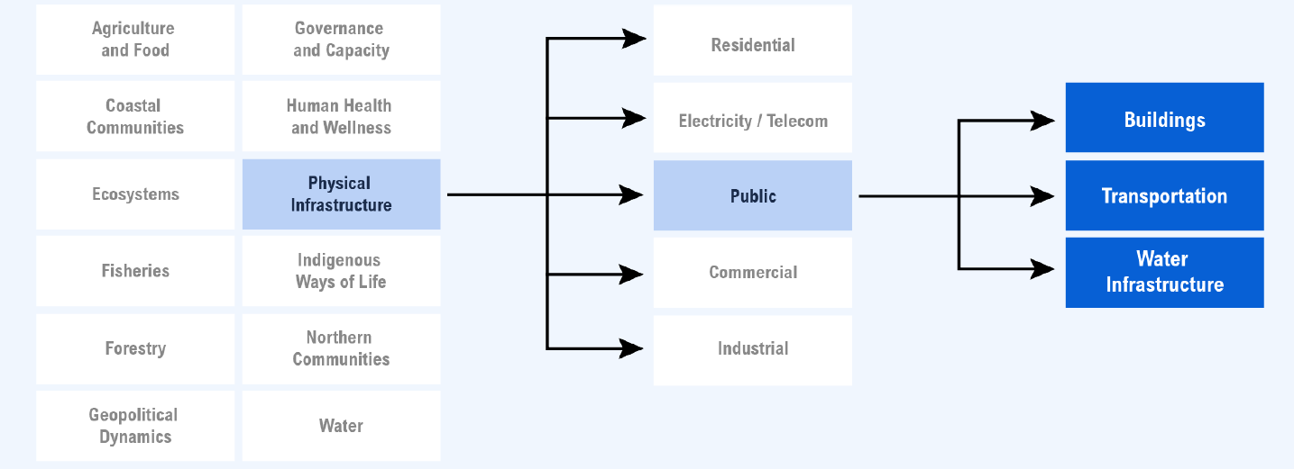
Source: Council of Canadian Academies and FAO.
To ensure safety and reliability, infrastructure is designed, built and maintained to withstand a specific range of climate conditions typically based on historic climatic loads. However, as many public assets are typically designed to last between 50 and 100 years, it is no longer feasible to rely on past climate parameters to design and manage public infrastructure,[6] as infrastructure in Canada faces significant risk from the impacts of climate change that are expected to reduce their lifespan and effectiveness.[7]
Project Context
- 2009
 Adapting to Climate Change in Ontario: Report of the Expert Panel on Climate Change Adaptation
- 2011
 Climate Ready: Ontario’s Adaption Strategy and Action Plan
- 2013
 Natural Resources Canada First Annual Report of the Adaptation Platform
- 2016
 Office of the Auditor General of Ontario Annual Report
 Ontario’s Climate Change Action Plan, 2016-2020
- 2017
 Infrastructure and Buildings Working Group: Adaptation State of Play Report
- 2018
 Perspectives on Climate Change Action in Canada: A Collaborative Report from Auditors General
 A Made-in-Ontario Environment Plan
- 2019
 Government of Canada: Canada’s Changing Climate Report
- 2020
 Government of Canada: Climate-Resilient Buildings and Core Public Infrastructure
- 2021
 Government of Canada: Canada in a Changing Climate – National Issues Report
Canada has produced a significant and growing body of work examining climate change and its potential impacts on public infrastructure. However, while the federal and Ontario climate plans have set emission targets and acknowledged the importance of funding infrastructure resilience,[8] neither government has fully assessed the climate risks to public infrastructure or developed comprehensive adaptation plans to address them.[9]
At the federal level, Canada’s Climate Change Adaptation Platform was established in 2012 as a national forum for disseminating information and promoting collaboration among stakeholders.[10] As part of the platform, the Infrastructure and Buildings Working Group (IBWG) produced an overview of the state of climate adaptation in Canada and has identified priorities for all governments, including the need to develop asset inventories and dedicate budgets to climate change adaptation.[11] The impact of climate change on design data[12] in Canada was also recently assessed under the Climate-Resilient Buildings and Core Public Infrastructure Initiative,[13] which could be integrated into national and provincial building codes as early as 2025.[14] The federal government’s National Issues Report also presented a nation-wide overview of climate change impacts and adaptation issues. The report highlights the importance of economic analysis to inform adaptation planning, and the benefits of adaptation and proactive investment.[15] The federal government’s National Adaptation Strategy, which will be developed in consultation with a broad range of stakeholders including provinces and territories, is slated for release in fall 2022.[16]
At the provincial level, Ontario’s Expert Panel on Climate Change Adaptation released a report in 2009 with recommendations for a province-wide climate change adaptation plan.[17] The Province released its first Climate Change Adaptation Strategy and Action Plan in 2011,[18] which adopted the recommendations and set broad goals for emissions reduction and climate change adaptation. However, the 2016 annual report from Ontario’s Auditor General noted that as of August 2016, many items from the 2011 Adaptation Plan were only partially carried out.[19] Subsequently, the Province released a five-year Climate Change Action Plan in 2016 that highlighted a handful of adaptation measures but did not explicitly follow up on the 2011 Adaptation Strategy.[20]
In 2015, Ontario passed the Infrastructure for Jobs and Prosperity Act, 2015, which contained 14 principles that the government and every broader public sector entity were required to consider when making infrastructure decisions, including resilience to the effects of climate change.[21] Under the same Act, Ontario passed the Asset Management Planning for Municipal Infrastructure regulation, which requires municipalities to consider actions to address possible infrastructure vulnerabilities to climate change.[22]
In November 2018, the government released an environment plan that promised to assess the impact of climate change to Ontario’s communities, critical infrastructure, economies and natural environment, and to conduct impact and vulnerability assessments for key sectors such as transportation and water. In its 2019 report on environmental issues in Ontario, the Office of the Auditor General of Ontario acknowledged that climate change will exacerbate infrastructure damage from extreme weather and identified that infrastructure resiliency in Ontario needs significant improvements.[23] In 2020, the Government of Ontario released its strategy to reduce the impacts and risks of flooding in the province.[24] Finally, Ontario launched its Climate Change Impact Assessment project in 2020, due for completion in 2022, which aims to evaluate climate change impacts at the provincial and regional scales in key areas, including infrastructure.[25]
Outside of government, the insurance industry evaluates the costs of the impacts of natural disasters to private infrastructure, often for singular events.[26] Many assessments of climate impacts to public infrastructure focus on specific assets, such as the Public Infrastructure Engineering Vulnerability Committee’s (PIEVC) case studies that examine the resilience of individual assets and asset components to climate scenarios.[27]
The Task Force on Climate-Related Financial Disclosures recommends that public and private asset managers assess and disclose physical climate risks for incorporation into financial decision making, but this is not yet common practice in Canada.[28] Recently, however, some institutions are beginning to conduct detailed assessments of the costs of climate change to public and private infrastructure at the national level.[29]
As such, the FAO’s CIPI project joins a growing literature on the impacts of climate change to public infrastructure.
The FAO’s “Costing Climate Change Impacts to Public Infrastructure” Project
In June 2019, a Member of Provincial Parliament asked the FAO to analyze the costs that climate change impacts could impose on Ontario’s provincial and municipal infrastructure, and how those costs could impact the long-term budget outlook of the province. In response to this request, the FAO launched its “Costing Climate Impacts to Public Infrastructure” project (CIPI).
In the first phase of the project, the FAO assessed the composition and state of repair of provincial infrastructure and released its findings in November 2020.[30] In the second phase, the FAO conducted a similar assessment of Ontario’s municipal infrastructure, with results released in August 2021.[31]
The purpose of the final phase of the CIPI project is to provide broad estimates of the long-term budgetary costs that certain climate change hazards could impose on the province and municipalities through accelerated infrastructure deterioration, increased operating expenses or compromised service levels, in the absence of adaptation measures. The project will also discuss adaptation options to address these climate hazards, and provide a broad range of costs estimates at the portfolio level.
It is well established that keeping assets in a state of good repair helps to maximize the benefits of public infrastructure in a cost-effective manner over time. Climate change will clearly impact public infrastructure in many ways that could carry significant budgetary consequences. While the concept of quantifying these impacts and estimating their financial liabilities for asset owners is relatively new, this methodology could support capital funding decisions by provincial and municipal governments now and into the future.
While public infrastructure faces many climate hazards, this project focuses on those that are likely to have the largest budgetary impact and can be projected by climate scientists with a reasonable degree of confidence. These hazards include extreme rainfall (pluvial flooding), extreme heat and freeze-thaw cycles. Chapter 2 describes the climate projections used in the project, their key trends, and the selection rationale for the project’s climate hazards.
Several issues go beyond the scope of this project. While greenhouse gas reduction is important, the CIPI project does not assess the Province of Ontario’s reduction efforts. The project also does not assess the climate resiliency of specific assets, but instead approaches the issue at an asset class level. The project focuses on the financial impacts to provincial and municipal asset managers and does not attempt to assess the societal impacts or costs of infrastructure failure.[32] As a result, the project does not conduct a cost-benefit analysis that compares climate change damage and adaptation costs. The project also does not assess the climate impacts to private infrastructure, including housing, commercial or industrial facilities. The methodology for the project including key caveats and assumptions is outlined in Chapter 3.
To complete the CIPI project, the FAO partnered with the Canadian Centre for Climate Services and WSP. WSP is a large engineering firm with expertise in all aspects of public sector infrastructure, including asset management, public infrastructure construction and operations, and climate change impacts. [33] The FAO contracted WSP to establish relationships between relevant climate indicators and key infrastructure costs (or “climate cost elasticities”, see Chapter 3 for a detailed discussion). The Canadian Centre for Climate Services provided the FAO with regional projections of the climate indicators specified by WSP engineers.
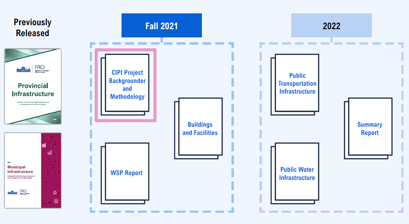
The third phase of the FAO’s CIPI project will be presented in six separate reports:
- CIPI Project Backgrounder and Methodology
- WSP Engineering Report, outlining the methodology and engineering rationale behind the “climate cost elasticities”
- Costing the Impacts of Extreme Rainfall, Extreme Heat and Freeze-Thaw Cycles to Public Buildings in Ontario
- Costing the Impacts of Extreme Rainfall, Extreme Heat and Freeze-Thaw Cycles to Public Transportation Infrastructure in Ontario
- Costing the Impact of Extreme Rainfall to Public Water Infrastructure in Ontario
- CIPI Project Summary Report
2 | Projecting Climate Hazards to Public Infrastructure
In a changing climate, infrastructure in Ontario faces increasing risks from numerous climate hazards, both from more frequent extreme events and from chronic impacts. The severity of these impacts in the future depends on the extent of temperature increases, which will be influenced almost entirely by how quickly global greenhouse gas emissions can be lowered. This chapter presents the global climate change scenarios used in this project and describes the Ontario-specific climate change data. The chapter then discusses the important climate hazards to public infrastructure in Ontario and the FAO’s rationale for scoping which hazards to include in the study. Lastly, for those hazards selected for study, this chapter outlines the specific climate variables used to proxy these hazards, discusses their key trends, and assesses the level of uncertainty associated with their trends.
Global Climate Change Scenarios
There is unequivocal evidence that the emission of greenhouse gases from human activity is the dominant cause of the unprecedented rise in global temperatures since the beginning of the industrial era.[34] Since the late 19th century, rising concentrations of greenhouse gases have contributed to a roughly 1.1°C increase in the annual global mean temperature.[35]
Figure 2-1 Global surface temperature has risen in line with cumulative carbon dioxide emissions
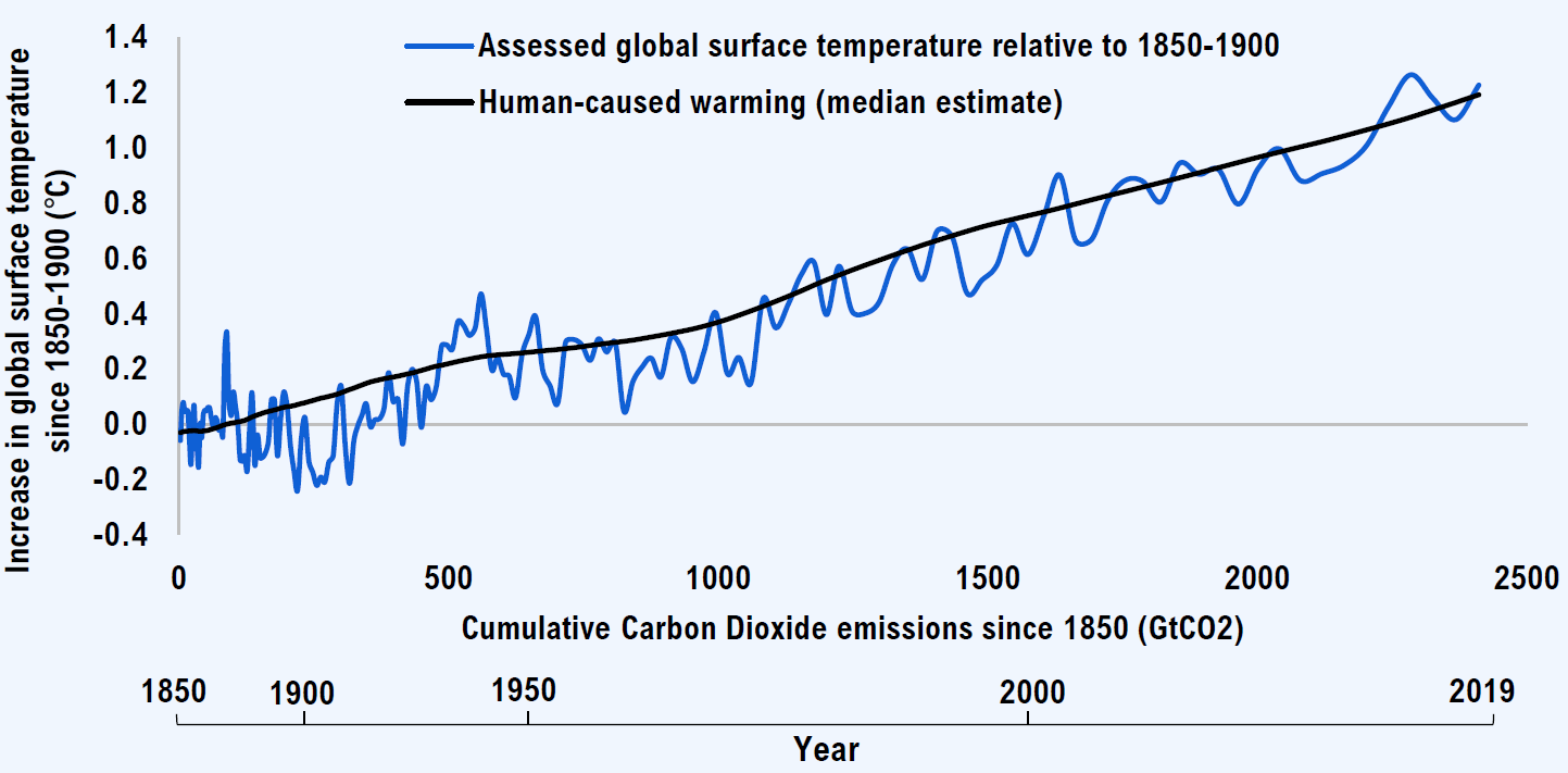
Source: Intergovernmental Panel on Climate Change.[36]
Rising global mean temperatures are leading to warmer ocean surface temperatures, the melting of Arctic sea ice, rising sea levels, heatwaves, droughts and a greater frequency of extreme weather events.[37]
The Intergovernmental Panel on Climate Change (IPCC) regularly produces assessments of climate change based on the latest climate data and scientific understanding. The physical science report of the IPCC’s sixth comprehensive assessment (AR6), released in August 2021, shows that the evidence of changes in climate extremes has strengthened since the previous assessment in 2013.[38]
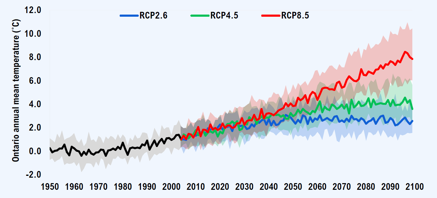
In the future, the extent of global temperature increases will be driven by global emissions, which in turn depend on the long-term rate of global population growth, economic growth, the amount and composition of energy use, and land use patterns, among other factors. The IPCC’s fifth comprehensive assessment (AR5)[39] produced four scenarios called Representative Concentration Pathways (RCPs). The RCPs are unique in their assumptions for future concentrations of greenhouse gases in the atmosphere, and each RCP is named after the level of “radiative forcing” by 2100.[40]
- RCP2.6: This is the “low emissions” scenario that assumes a major and immediate turnaround in global climate policies. Emissions are projected to peak in the early 2020s and decline to zero by the 2080s due to stringent climate policy. By the end of the century, net emissions are negative. In this scenario, global mean temperatures are projected to increase around 0.8 to 2.4°C by 2100 compared to the pre-industrial average (to account for the uncertainty between climate models, all projections of climate variables are presented as ranges).[41]
- RCP4.5: This is a “medium emissions” scenario, where global emissions are assumed to peak in the 2040s, decline rapidly over the following four decades, and then stabilize at the end of the century. Global mean temperatures are projected to increase around 1.7 to 3.2°C by 2100 compared to the pre-industrial average.
- RCP6.0: This is a somewhat higher “medium emissions” scenario, where global emissions are projected to peak in the 2080s and decline over the following two decades. Global mean temperatures are projected to increase around 2.1 to 3.8°C by 2100 compared to the pre-industrial average.
- RCP8.5: This is the “high emissions” scenario that assumes no meaningful change in global climate policies. Emissions are projected to continue growing at the current pace for most of the century. Global mean temperatures are projected to increase around 3.2 to 5.4°C compared to the pre-industrial average.
Cumulative emissions from 2005 to 2020 most closely match the RCP8.5 scenario.[42]
Figure 2-2 Increase in global mean temperature relative to 1850-1900
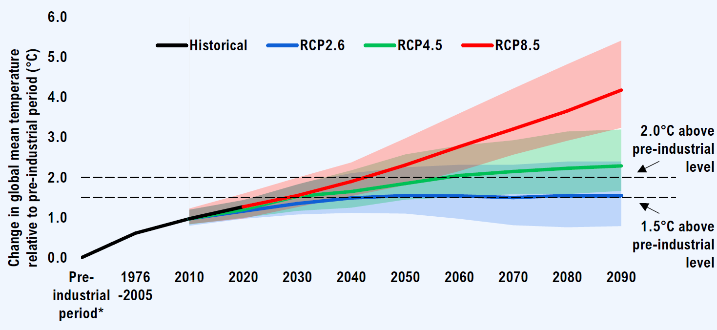
* 1850-1900 base period.
Note: Shaded areas show the range of 5th and 95th percentile projections.
Source: Intergovernmental Panel on Climate Change.[43]
The Paris Agreement (2016) set targets to prevent the increase in global mean temperatures to well below 2.0°C above pre-industrial levels, with efforts to limit the increase to 1.5°C. According to the IPCC, even a 1.5°C increase in global mean temperatures compared to pre-industrial levels would still be associated with significant negative consequences to human health, food and water availability, and vulnerable ecosystems.[44]
Under all RCP scenarios, global temperatures are likely to rise by 1.5°C or more by 2040 relative to pre-industrial levels. Even in the lowest emissions scenario, further warming is irreversible by mid-century. This means that even if greenhouse gas concentrations and the global mean temperature stabilize by mid-century, sea levels will continue to rise, ice will continue to melt, and extreme weather events are expected to increase in frequency. This is partially due to challenges in reducing atmospheric greenhouse gas concentrations, and partially because the oceans and ice sheets take a very long time to adjust to new surface temperatures. Beyond 2040, the pace of climate change will depend on future emissions and global efforts to curb them.
There are no probabilities assigned to the RCPs, but the remaining global “carbon budget” (the total amount of greenhouse gases that could be emitted while staying below 1.5°C above pre-industrial levels) is rapidly depleting. Among the IPCC scenarios, only the RCP2.6 is within the range of a global mean temperature increase below 1.5°C,[45] roughly in line with the Paris Agreement. Under RCP4.5, global mean temperatures rise 1.5 to 2.8°C above pre-industrial levels in the 2060s, reaching 1.7 to 3.2°C by 2100.
Climate Change Data Used in CIPI
Although climate processes are closely interconnected around the world, global models project climate variables at a broad spatial scale. To incorporate variations in geographic features at the regional level, these global projections must be “downscaled” to facilitate climate change projections at finer spatial resolutions.
To ensure that the project used credible climate projections, the FAO partnered with the Canadian Centre for Climate Services (CCCS), an office within Environment and Climate Change Canada dedicated to assisting partners with climate data needs, among other functions.[46] The CCCS[47] produced climate projections using the BCCAQv2 dataset,[48] a widely recognized source that has been transparently peer reviewed and used extensively in Canada, including in Canada’s Changing Climate Report,[49] the data available on ClimateData.ca, and the Climate Atlas of Canada.[50] Source code and resulting data are available upon request to the CCCS.
The following sections discuss the CCCS data in terms of the RCP scenarios and projection uncertainty, regional projections, and the historical baseline used in the CIPI project, and then compare future projections of Ontario’s mean temperature with that of the global mean.
RCP Scenarios and Climate Projection Uncertainty
CCCS projections were available for RCP2.6, RCP4.5 and RCP8.5 scenarios but not for RCP6.0.[51] For the three RCP scenarios, the CCCS provided projections from 24 of the global models supporting the IPCC’s fifth Assessment Report (AR5).[52] Within each RCP scenario for future global greenhouse gas concentrations, each of these 24 models have somewhat different projections of climate variables due to natural variability and different assumptions for climate processes for which there are scientific uncertainties.[53] To account for the uncertainty surrounding the earth’s future climate response in each RCP, the CCCS provided the median (50th percentile) projection, the 90th percentile projection (which 90 per cent of model results fall below) and the 10th percentile projection (which 10 per cent of model results fall below) from the ensemble of 24 global models.
Over the past 10 years, global emissions have followed RCP8.5 most closely,[54] although controlling warming to less than 1.5°C is still possible to achieve through immediate and aggressive action. To simplify the presentation in subsequent FAO costing reports, the CIPI project will largely focus on projections from the RCP4.5 and RCP8.5 scenarios, and present impacts under RCP2.6 as background information.[55]
CCCS Regional Climate Projections
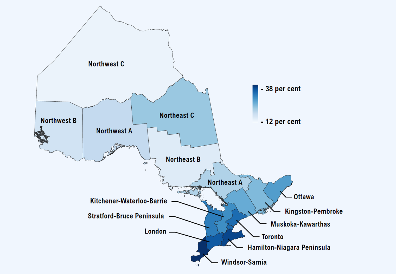
Regional variation in climate change means that infrastructure located in southern Ontario will experience different impacts compared to that located in northern Ontario. With the assistance of the CCCS, it was determined that averaging the climate change projections into 15 regions in Ontario would adequately capture regional variability. These regions were defined using Statistics Canada’s definition of economic regions,[56] with the northeast and northwest regions each divided into three sub-regions due to their size and climate variability.
Figure 2-3 Climate projections produced for CIPI capture variations across 15 economic regions in Ontario
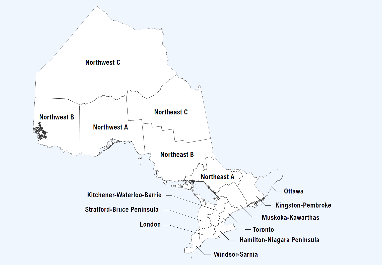
Source: Statistics Canada, FAO.
Within each region, the CCCS produced projections for all the climate variables required by the CIPI project, for all three RCP scenarios. For all indices except extreme precipitation indices, the daily climate data were processed on a per-model, per-climate scenario, per-grid cell basis to develop annual index time series for all BCCAQv2 grid cells falling within each economic region. Following this processing, aggregate values were determined on an annual basis and in sliding 30-year windows for each scenario and economic region.
Extreme precipitation indices were calculated on a station-by-station basis, for all Environment and Climate Change Canada intensity-duration-frequency (IDF) station locations.[57] Observed (historical) extreme precipitation indices at these stations were scaled according to the annual climatological (30-year) temperature change at the corresponding location using the Clausius–Clapeyron temperature-based scaling approach.[58]
In general, the moisture-holding capacity of air increases as the air warms. The relationship between temperature and the atmosphere’s water-holding capacity is described by the Clausius–Clapeyron relation, which indicates that extreme precipitation is expected to increase by around 7 per cent for every 1°C increase in mean temperature.[59]
Once the station-based IDF curves were projected, the results were aggregated to the economic region level, and representative station values were determined for the 10th, 50th and 90th percentiles of station values within each economic region.
Historical Baseline for the CIPI Project
To assess human influence on the global climate, the IPCC typically compares emissions and temperature increases relative to the pre-industrial era, defined as the 1850-1900 period (see charts 2-1 and 2-2 above). However, the purpose of the CIPI project is to assess how changes in climate variables in the future could impact infrastructure costs relative to the recent past. Consequently, the historical baseline for CIPI is defined as the 1976-2005 period, as a significant portion of Ontario’s current public infrastructure was built and designed to the climate of that period, and because the CCCS’s regionally downscaled climate data in Ontario are available from 1950. All further climate analytics in this report and in subsequent reports will use the 1976-2005 period as the historical baseline.[60]
Ontario’s Mean Temperature Projected to Rise Faster than the Global Mean
CCCS projections show that Ontario’s annual mean temperature will have increased by around 1.6°C between 1950 and 2019, faster than the global average rate of warming.[61] This trend reflects faster warming near the earth’s poles in part due to regional climate feedbacks.[62] Also, temperature in Ontario has increased more in winter than in warmer seasons.[63] The proportion of precipitation falling as snow has declined significantly, and the replacement of snowfall by rain has affected river and stream flows.[64] Other observed changes in Ontario include decreases in snow cover and seasonal snow accumulation, earlier ice breakup and later freeze-up in lakes.
Ontario’s mean temperature will continue to rise at a faster pace than the global mean due to the same climate feedbacks observed in the past. For example, in the RCP8.5 scenario the global mean temperature is projected to rise by 1.3 to 2.5°C by mid-century compared with the 1976-2005 average,[65] which translates to a 2.8 to 4.9°C increase in Ontario’s annual mean temperature.[66]
Figure 2-4 Ontario’s mean temperature projected to rise faster than global mean temperature under RCP8.5
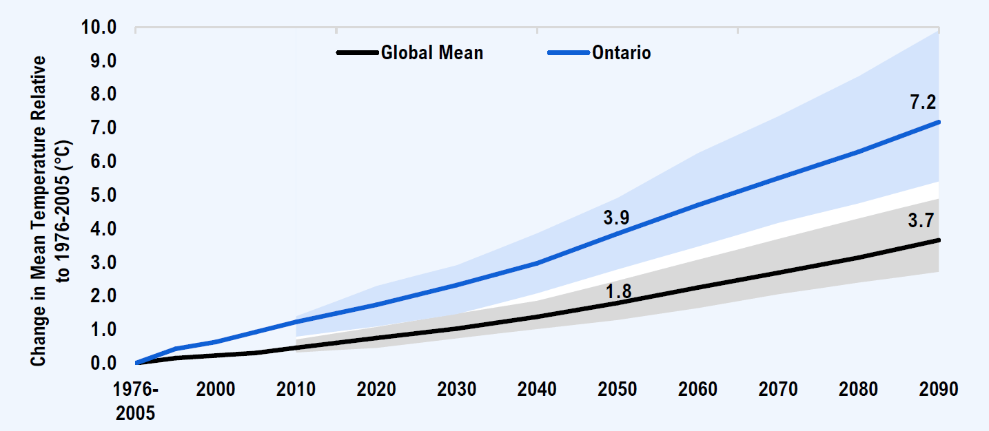
Note: Shaded areas show the range of 5th and 95th percentile projections for the global mean, and the range of 10th and 90th percentile projections for Ontario.
Source: Intergovernmental Panel on Climate Change[67] and Canadian Centre for Climate Services.
Scope of Climate Hazards in CIPI
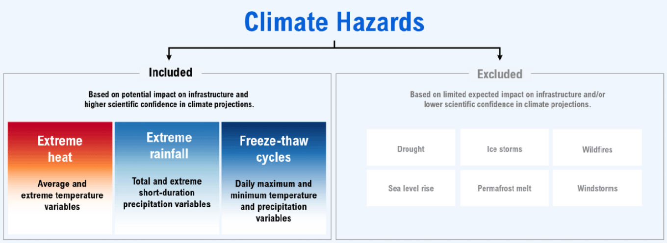
Climate change is associated with many hazards to public infrastructure, which can take the form of extreme weather events or long-term trends that can impact asset depreciation. Ontario has been subject to costly floods and ice storms and is also prone to droughts, intense rainfall, wildfires, windstorms, heat waves and permafrost melt.[68] It was not possible to include all climate hazards to public infrastructure in this report due to the availability of credible projections, the relevance of specific hazards to provincial and municipal infrastructure (see Chapter 3: “Scope of Public Infrastructure Assets Included in CIPI”), and the FAO’s own resource constraints. In deciding which climate hazards to include, the FAO chose to focus on those with broad and material impacts on provincial and municipal infrastructure, and those with a strong link to climate variables that can be projected with reasonable scientific confidence. This section briefly reviews the major hazards relevant to public infrastructure in Ontario and presents the rationale for the scope of hazards included in the CIPI project.
Extreme heat events are extended spells of high temperatures that cause surface damage to buildings and roads, and accelerate the deterioration of transportation infrastructure. As extreme high temperatures increase in frequency and duration, heatwaves will intensify. Given the high scientific confidence[69] attached to temperature projections and the potential impact on a wide range of public infrastructure, this hazard is included in the CIPI project.
Wildfires have multiple causes of ignition and are exacerbated by dry, windy conditions and hot temperatures. In severe cases where population centres are affected, wildfires can damage and destroy all types of infrastructure. Projecting the future risk of wildfires is challenging due to the complex interplay between temperature and precipitation variables, and there is high uncertainty in how changes in these variables could affect forest moisture content or the drivers of ignition. As a result, this hazard is not included in the CIPI project.
Extreme rainfall, or intense precipitation over a short period, can cause water damage to buildings and strain water and stormwater infrastructure. Extreme rainfall will become more common as short-duration precipitation increases. Since heavy rainfall is directly represented by extreme precipitation variables and holds significant impact on a wide range of infrastructure, this hazard is included in the CIPI project.
- Note that while the impacts of pluvial flooding are included in this hazard, the impacts of flooded rivers (i.e., fluvial flooding) are not included due to the complex connection between extreme rainfall and fluvial flooding and the lack of publicly accessible flood plain mapping for many of Ontario’s drainage basins.
Ice storms, or extreme freezing precipitation, can damage buildings and transportation infrastructure, and increase structural loads with ice buildup. Total precipitation is projected to increase, but the rise in average temperatures and shorter cold seasons leads to an ambiguous trend for future ice storms. Climate data related to snow load and ice accretion are also subject to low scientific confidence. Given these considerations, this hazard is excluded from the CIPI project.
Windstorms can damage cladding and roofs. Since historical observations for short-duration wind pressures and wind speed are limited and subject to low scientific confidence,[70] windstorms are excluded from the CIPI project.
Droughts are extended periods of below-average precipitation, sometimes accompanied by elevated temperatures, which can strain infrastructure by increasing water demands. The rise in average temperatures could lead to more widespread and frequent droughts, but also to an increase in average and extreme precipitation.[71] Droughts are only partially linked to extreme temperature variables and could have limited impact on most types of public infrastructure, so they are excluded from the CIPI project.
Permafrost degradation can compromise building foundations and roads, and rupture underground pipes. The share of provincial and municipal infrastructure located in permafrost areas is small, but the consequences of these impacts could be significant for communities in Ontario’s Far North. While there is high scientific confidence in projections for mean air temperature increases over Ontario’s large permafrost areas, there is less confidence in projecting the associated reductions in permafrost extent due to inadequate representation of soil properties in climate models.[72] Consequently, this hazard was excluded from the CIPI project. Similarly, while the impacts of rising sea levels in Hudson Bay will be very significant for Northern communities, this hazard was excluded due to the small share of provincial and municipal infrastructure located in these areas.
Finally, freeze-thaw cycles are fluctuations between freezing and non-freezing air temperatures that impact a wide range of infrastructure. These temperature changes can damage building structures and envelopes as well as bridges. When combined with increases in precipitation that can soak into road bases, such temperature changes can also cause significant damage to roads. While freeze-thaw cycles are challenging to project in part because they require combining multiple climate variables (see discussion on page 22), the underlying temperature and precipitation data come with a high degree of scientific confidence. Therefore, this hazard is included in the CIPI project.
In summary, the FAO’s CIPI project focuses on extreme heat, extreme rainfall and freeze-thaw cycles. These three climate hazards may have broad and financially material impacts on public infrastructure and can be projected using climate variables that have a high degree of scientific confidence.
Key Trends in Temperature, Rainfall and Freeze-Thaw Cycles in Ontario
The future change in climate hazards to public infrastructure can be proxied by examining projections for specific climate variables. For each of the three climate hazards in CIPI’s scope, there are many climate indicators to choose from. This section outlines some of the key climate indicators used in the CIPI project to proxy the three hazards, their key trends in Ontario and the level of confidence associated with those trends. Chapter 3 discusses how these projections are used to estimate changes in infrastructure costs, and WSP’s report presents the engineering rationale for selecting the most appropriate climate indicator for each specific use.
Extreme Heat
All RCP scenarios project that Ontario will be warmer in the future. However, projected changes in Ontario mean temperatures differ significantly in the low and high emission scenarios. Compared to the 1976-2005 average, annual mean temperatures in Ontario over the 2071-2100 period are projected to be 2.0°C (1.4 to 3.1°C)[73] higher under RCP2.6, 3.3°C (2.2 to 4.9°C) higher under RCP4.5, and 6.3°C (4.8 to 8.5°C) higher under RCP8.5.
Figure 2-6 Annual mean temperature, Ontario average
Note: Shaded areas show the ranges of 10th and 90th percentile projections.
Source: Canadian Centre for Climate Services.
Temperatures are expected to rise faster in northern Ontario than in southern Ontario due to regional climate feedbacks such as the decrease in snow and ice reflectivity. In northern Ontario under RCP8.5, annual mean temperature over the 2071-2100 period is projected to rise by 6.7°C (5.0 to 8.8°C), compared to an increase of 5.6°C (4.3 to 6.9°C) in the Windsor-Sarnia region. While southern Ontario is projected to warm slightly slower than northern Ontario, it is still warming faster than the global mean. In addition, winter mean temperatures in Ontario are rising faster than summer mean temperatures.
Figure 2-7 Median projected change in annual mean temperatures from 1976-2005 to 2071-2100, RCP8.5
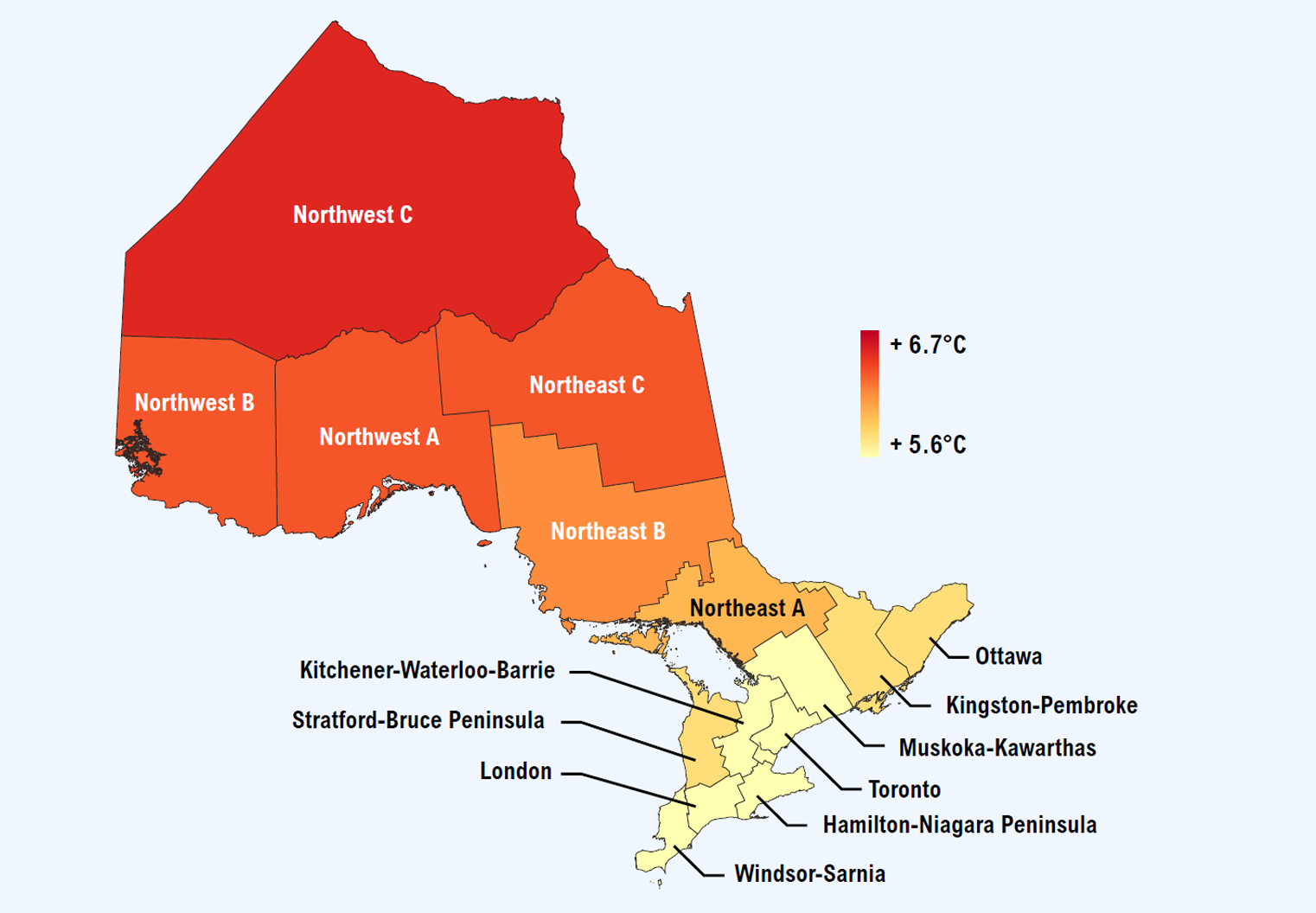
Note: Colour distribution is based on the multi-model median projection.
Source: Canadian Centre for Climate Services.
Daily extreme temperatures will increase at a similar pace as mean temperatures. Compared to the 1976-2005 average, annual highest daily maximum temperatures over the 2071-2100 period are projected to be 2.0°C (0.9 to 2.8°C) higher under RCP2.6, 3.4°C (2.3 to 4.2°C) higher under RCP4.5, and 6.5°C (4.1 to 7.5°C) higher under RCP8.5.
Hot temperature extremes will last longer and occur more frequently. Compared to the 1976-2005 average, the annual number of hot days[74] is projected to increase by 5 days (2 to 10 days) under RCP2.6, 13 days (6 to 18 days) under RCP4.5, and 34 days (17 to 46 days) under RCP8.5 by 2071-2100. Similarly, cooling degree days[75] are projected to increase by 71°C-days (37 to 117°C-days) under RCP2.6, 161°C-days (86 to 212°C-days) under RCP4.5, and 381°C-days (225 to 515°C-days) under RCP8.5.
| Variable | Definition | RCP2.6 | RCP4.5 | RCP8.5 |
|---|---|---|---|---|
| Annual mean daily temperature | Annual mean temperature estimated from daily temperatures | +2.0°C (+1.4 to 3.1°C) |
+3.3°C (+2.2 to 4.9°C) |
+6.3°C (+4.8 to 8.5°C) |
| Annual number of hot days | Annual number of days with daily maximum temperature above 30°C | +5 days (+2 to 10 days) |
+13 days (+6 to 18 days) |
+34 days (+17 to 46 days) |
| Highest annual temperature | Annual highest daily maximum temperature | +2.0°C (+0.9 to 2.8°C) |
+3.4°C (+2.3 to 4.3°C) |
+6.5°C (+4.1 to 7.5°C) |
| Mean July maximum daily temperature | Monthly mean of daily maximum temperature in July | +1.8°C (+0.9 to 2.5°C) |
+3.6°C (+1.9 to 3.8°C) |
+6.5°C (+4.0 to 7.9°C) |
| 2.5% July daily maximum temperature | 97.5th percentile of the distribution of daily maximum temperature in July | +1.9°C (+0.9 to 2.8°C) |
+3.4°C (+2.4 to 4.3°C) |
+6.5°C (+4.3 to 7.6°C) |
| Annual number of cooling degree-days | Annual sum of daily degrees above 18°C | +71°C-days (+37 to 117°C-days) |
+161°C-days (+86 to 212°C-days) |
+381°C-days (+225 to 515°C-days) |
In general, there is high confidence in the projected trends and ranges of temperature variables based on strong scientific evidence in the causes of observed changes.[76]
Extreme Rainfall
Annual mean precipitation has increased in Ontario and Canada since the mid-20th century. From 1948 to 2012, Ontario’s annual mean precipitation increased 9.7 per cent, compared to 18.3 per cent for all of Canada.[77] For extreme rainfall over shorter timescales, observations have been inconsistent. For example, short-duration extreme precipitation, such as the volume of rainfall within a 24-hour timespan, has not followed a detectable trend.[78]
Total precipitation in Ontario is projected to increase. Compared to the 1976-2005 average, annual total precipitation over the 2071-2100 period is projected to be 7.1 per cent (4.0 to 7.8 per cent) higher under RCP2.6, 9.8 per cent (4.4 to 10.3 per cent) higher under RCP4.5, and 15.0 per cent (6.2 to 18.2 per cent) higher under RCP8.5. Since precipitation is generally lower in the north than in the south, the percentage increase in mean precipitation is greater in northern Ontario.
Figure 2-8 Total annual precipitation, Ontario average
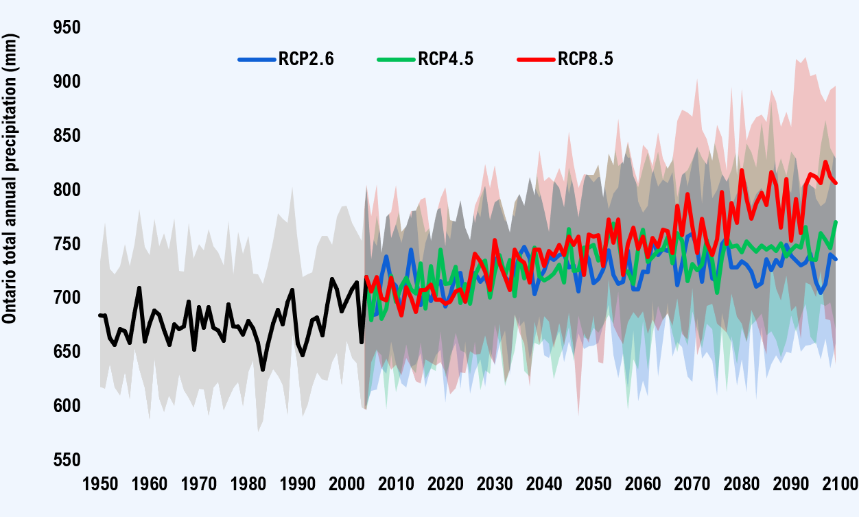
Note: Shaded areas show the range of 10th and 90th percentile projections.
Source: Canadian Centre for Climate Services.
Figure 2-9 Median projected change in total annual precipitation from 1976-2005 to 2071-2100 in RCP8.5
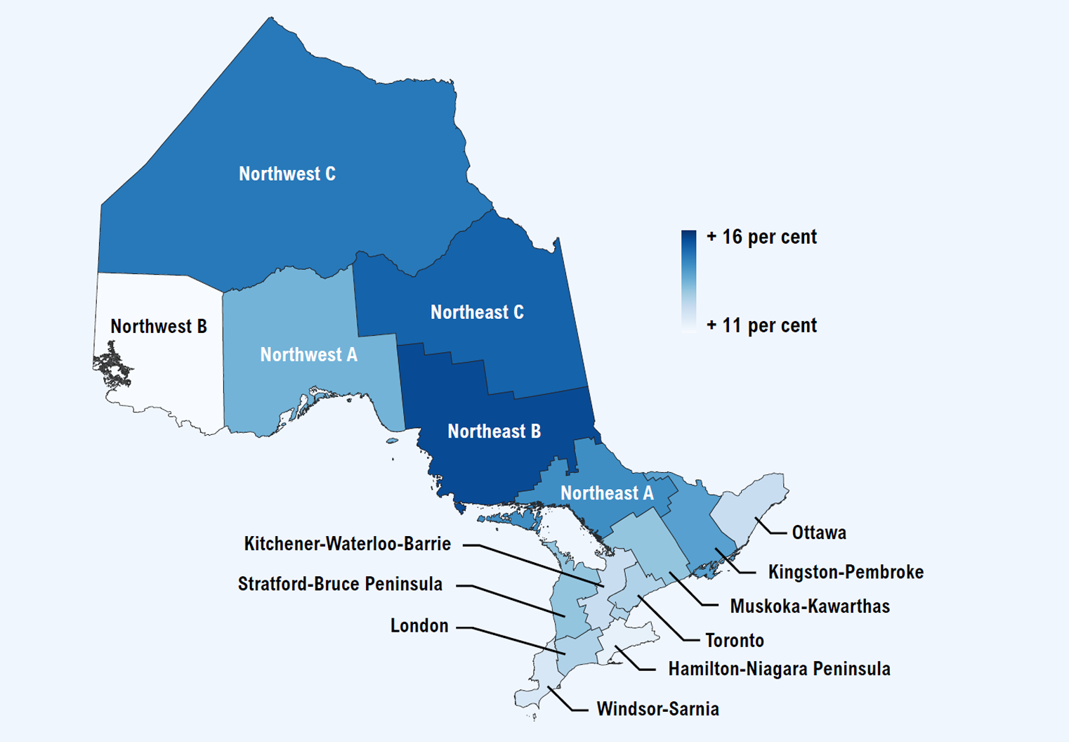
Note: Colour distribution is based on multi-model median projections.
Source: Canadian Centre for Climate Services.
Consistent with the increase in total precipitation, short-duration extreme precipitation is also expected to intensify. Intensity-duration-frequency (IDF) curves are graphical representations of the probability that a given rainfall intensity will occur. They play an important role in water resources engineering to describe the magnitudes of extreme rainfall events (e.g., the 100-year event) and to assist in designing urban drainage systems. For example, the IDF 15-minute 1:10 would show the maximum rainfall intensity in 15 minutes that is expected to occur in a 10-year period.
CCCS projections indicate that all historical IDF rainfall intensities will increase by 14.6 per cent (9.8 to 23.5 per cent) by late century relative to the 1976-2005 period under RCP2.6, by 24.9 per cent (16.1 to 39.4 per cent) under RCP4.5, and by 53.0 per cent (38.0 to 78.2 per cent) under RCP8.5.
| Variable | Definition | RCP2.6 | RCP4.5 | RCP8.5 |
|---|---|---|---|---|
| Annual total precipitation | Annual total amount of precipitation received | +7.1 (+4.0 to 7.8) |
+9.8 (+4.4 to 10.3) |
+15.0 (+6.2 to 18.2) |
| Maximum 5-day precipitation | Maximum amount of precipitation within a year received during five consecutive days | +8.7 (+7.6 to 11.5) |
+11.0 (+9.3 to 13.6) |
+18.7 (+12.5 to 19.5) |
| IDF 15-min 1:10 | Short duration rainfall intensity for a 15-minute 1-in-10-year event | +14.6 (+9.8 to 23.5) |
+24.9 (+16.1 to 39.4) |
+53.0 (+38.0 to 78.2) |
| IDF 24-hour 1:2 | Short duration rainfall intensity for a 24-hour 1-in-2-year event | +14.6 (+9.8 to 23.5) |
+24.9 (+16.1 to 39.4) |
+53.0 (+38.0 to 78.2) |
| IDF 24-hour 1:5 | Short duration rainfall intensity for a 24-hour 1-in-5-year event | +14.6 (+9.8 to 23.5) |
+24.9 (+16.1 to 39.4) |
+53.0 (+38.0 to 78.2) |
| IDF 24-hour 1:10 | Short duration rainfall intensity for a 24-hour 1-in-10-year event | +14.6 (+9.8 to 23.5) |
+24.9 (+16.1 to 39.4) |
+53.0 (+38.0 to 78.2) |
| IDF 24-hour 1:100 | Short duration rainfall intensity for a 24-hour 1-in-100-year event | +14.6 (+9.8 to 23.5) |
+24.9 (+16.1 to 39.4) |
+53.0 (+38.0 to 78.2) |
Projections of aggregate precipitation variables (annual total precipitation and maximum 5-day precipitation) are associated with high-to-medium confidence. All model projections point to a positive trend in these variables, but the climate processes involved are more uncertain[80] than for temperature variables.
For extreme precipitation variables (IDF variables), there is medium confidence in Ontario average projections, but the regional projections have additional uncertainties for extreme rainfall at specific locations over short time periods. As historical IDF curves alone cannot be used to assess future extreme rainfall, it was determined that temperature scaling using the Clausius–Clapeyron relation is a useful basis for projecting these variables; however, the approach is subject to regional uncertainties.
Freeze-Thaw Cycles
Freeze-thaw cycles (FTCs) at their most basic are fluctuations in air temperature between freezing and non-freezing temperatures. Under these conditions, water residing on surfaces or absorbed by infrastructure materials can quickly change between liquid and solid states. Since water expands as it freezes, the repeated expansion and contraction can damage infrastructure.
In this basic definition, annual FTCs can be defined as the number of days in a year with a daily maximum temperature above 0°C and a daily minimum temperature below 0°C. Using this definition, FTCs averaged 79 days in the 1950s and 76 days in the 2000s. As the winter season shortens due to climate change, this trend is projected to continue, with Ontario average FTCs declining by 4 days (0 to 12 days) under RCP2.6, 9 days (0 to 15 days) under RCP4.5, and 12 days (0 to 19 days) under RCP8.5 by late century compared to the 1976-2005 period.
Figure 2-10 Annual number of freeze-thaw cycles, Ontario average
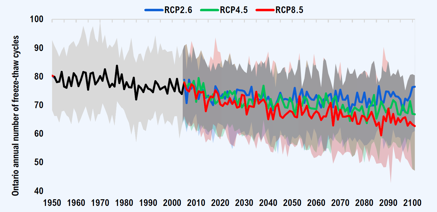
Note: Shaded areas show the range of 10th and 90th percentile projections.
Source: Canadian Centre for Climate Services.
Trends in FTCs vary significantly across Ontario regions. The decline in FTCs is more significant in southern Ontario where daily minimum temperatures will increasingly trend above 0°C. The large per cent change in southern Ontario relative to northern Ontario is due to the smaller number of FTCs in the current climate, which means that a similar level change as in the north results in a larger per cent change.
Figure 2-11 Median projected change in annual freeze-thaw cycles from 1976-2005 to 2071-2100, RCP 8.5
Note: Colour distribution is based on multi-model median projections.
Source: Canadian Centre for Climate Services.
The impact of FTCs may differ depending on their length and depth. For example, an FTC occurring in spring when the temperature dips below zero briefly during an otherwise warmer period could have less impact on infrastructure than an FTC that occurs in the depth of winter, when the temperature might crest above zero before a stretch of very low temperatures. “Deep” FTCs typically occur in winter, and are defined as those that occur when the daily average temperature is less than 0°C.
Overall, deep FTCs are declining in most regions of Ontario and in most scenarios. However, some scenarios show an increasing trend in Ontario’s northern regions as warmer winters reduce periods of deep freeze and increase periods of near 0°C temperatures. As such, Ontario average trends in deep FTCs range between significant decreases to significant increases (see Table 2-3).
Projecting the effect of FTCs on public infrastructure is more complex than merely projecting changes in their frequency. Changes in soil temperature and moisture content, as well as the amount of precipitation in winter, will also affect the stress and damage to infrastructure produced during FTCs.
WSP engineers indicated that the strictly temperature-based definitions of FTCs were a suitable proxy for the damage that could occur on infrastructure with vertical surfaces where less moisture would accrue (i.e., building envelopes or bridges). However, for horizontal assets including road pavement, the moisture content of the road base is also expected to contribute to the impact of FTCs.
Climate variables associated with humidity and moisture are subject to low scientific confidence due to challenges with measuring ground moisture content.[81] To better incorporate the effect of precipitation and moisture, WSP engineers indicated that the precipitation intensity in winter was the closest proxy to the moisture content of a road base in winter, and a relevant indicator for road pavement damage from FTCs. This is because rising rainfall intensity in winter will more frequently exceed the drainage capacity of roads, leading to more water penetration in the road base.
Winter rain intensity can be defined as the average amount of precipitation that occurs as rain[82] per day in winter.[83] Winter rain intensity in this definition is expected to increase by 5.8 per cent (1.5 to 7.0 per cent) in Ontario by late century compared to the 1976-2005 average under RCP2.6, by 10.5 per cent (2.6 to 13.0 per cent) under RCP4.5 and by 21.7 per cent (15.8 to 30.9 per cent) under RCP8.5.
Figure 2-12 Median winter rain intensity, Ontario average
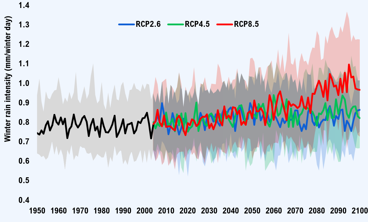
Note: Shaded areas show the range of 10th and 90th percentile projections.
Source: Canadian Centre for Climate Services.
WSP engineers indicated that trends in deep FTCs and trends in winter rain intensity are both relevant to projecting FTC damage to roads. To capture the trend of both indicators, WSP engineers proposed to create an index of road pavement damage from FTCs. However, while both indicators may be important to FTC damage on roads, WSP was not aware of any research to inform which indicator was more important. In the absence of any guidance on this issue, WSP proposed to weigh the trends in winter rain intensity and deep FTC events equally in the index. Table 2-3 summarizes the key FTC indicators used in this study.
| Variable | Definition | RCP2.6 | RCP4.5 | RCP8.5 |
|---|---|---|---|---|
| Annual freeze-thaw cycles | Annual number of days with daily maximum temperature above 0°C and daily minimum temperature below 0°C | -5.5 (-15.2 to 0.0) |
-12.1 (-19.2 to 0.0) |
-15.1 (-24.9 to 0.0) |
| Deep freeze-thaw cycles | Annual number of days with daily maximum temperature above 0°C, daily minimum temperature below 0°C, and daily average temperature equal or less than 0°C | -2.3 (-8.3 to +4.6) |
-4.4 (-10.8 to +4.8) |
-4.9 (-15.8 to +12.5) |
| Winter days | Total numbers of days in a year from January 1st to the last spring frost (last day in the year before July 1st where the daily minimum temperature was below 0°C) plus the number of days from first fall frost (first day in the year after July 1st where the daily minimum temperature was below 0°C) to December 31st | -17 days (-38 to -13 days) |
-29 days (-54 to -26 days) |
-55 days (-75 to -47 days) |
| Winter rain | Annual precipitation that occurs when the daily mean temperature is above 0°C, summed over winter days as defined above | -3.9 (-16.3 to +2.5) |
-4.5 (-21.8 to -2.2) |
-6.4 (-18.4 to +0.1) |
| Winter rain intensity | The amount of winter rain per “winter day” as defined above (mm/day) | +5.8 (+1.5 to 7.0) |
+10.5 (+2.6 to 13.0) |
+21.7 (+15.8 to 30.9) |
| FTC damage index for roads | 0.5 * per cent change in Deep FTCs + 0.5 * per cent change in winter rain intensity | +1.7 (-3.4 to 5.8) |
+3.0 (-4.1 to 8.9) |
+8.4 (0.0 to 21.7) |
There is high confidence in the projections of annual FTCs and medium confidence in deep FTCs based on the amount of evidence for projected trends and ranges. While annual FTCs are projected to decline in all regions and scenarios, deep FTCs are projected to increase in Ontario’s northern regions in some scenarios.
Projections of winter rain intensity are associated with medium confidence.[84] As temperatures rise, the number of winter days is declining in all regions and scenarios due to the shortening winter period. At the same time, winter rain intensity is increasing in all scenarios and regions. On balance, the combination of these trends leads to a declining volume of winter rain in most regions and scenarios.
Finally, there is lower confidence in the projection for the FTC road damage index due to the lack of research informing how the trends in deep FTCs and winter rain intensity should be combined.
3 | CIPI Methodology
Summary
In the first two phases of the CIPI project, the FAO estimated the state of repair of Ontario’s provincial and municipal infrastructure assets. The purpose of the final phase of the CIPI project is to provide broad estimates of the long-term budgetary costs that certain climate change hazards could impose on the province and municipalities through accelerated infrastructure deterioration and increased operating expenses.
This chapter begins by describing the scope of public infrastructure assets to be included in the third phase of the project. The chapter then briefly describes the infrastructure deterioration model, and how it is used to project the cost of maintaining public infrastructure in a state of good repair over the long term. This forms the base case against which to compare scenarios that include climate change impacts.
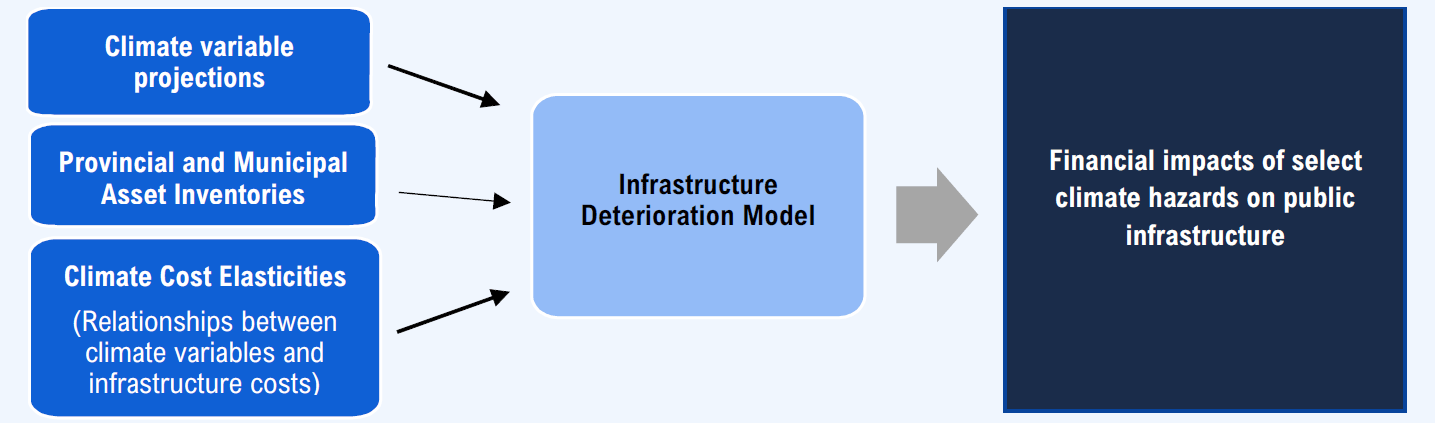
The next section describes how the scenarios with climate change impacts were constructed. The “costs of climate change” to public infrastructure can include both damage costs and costs associated with adaptation actions. Both types of costs are incorporated into the infrastructure deterioration model using broad engineering relationships developed by WSP. These relationships are called “climate cost elasticities” and relate changes in key climate variables to changes in various types of infrastructure costs. These costs are defined and described, and a brief outline of WSP’s climate cost elasticities is provided.[85]
Finally, this chapter outlines the important uncertainties involved in projecting the financial impact of changing climate hazards to public infrastructure. The chapter also discusses some key strengths, limitations, and caveats of the FAO’s approach.
Scope of Public Infrastructure Assets Included in CIPI
Public infrastructure in Ontario is owned by three levels of government: the Government of Canada, the Government of Ontario, and Ontario’s municipalities.[86] In the first two phases of the CIPI project, the FAO analyzed the state of repair of infrastructure assets owned by the Province and Ontario’s municipalities.[87] In the process, the FAO developed detailed asset databases containing $220 billion of provincial assets[88] and $484 billion of municipal assets.
The scope of assets in those reports did not include:
- federal infrastructure or infrastructure owned by crown corporations (like electricity generation/ distribution or casinos);
- land, forestry and information technology assets; and
- certain municipal infrastructure due to data availability limitations, including municipal machinery and equipment assets and certain types of municipal engineering infrastructure.
Within the scope of these assets, the FAO worked with WSP to establish which climate hazards could have the most significant impact on which asset classes. As each hazard would interact with each asset class in a different way, it was agreed that WSP would focus attention on the “interactions” that could present the greatest financial impact to asset managers. WSP’s assessment determined that the CIPI project should focus on the 12 most significant interactions
Figure 3-2 Scope of interactions between selected climate hazards and public asset classes
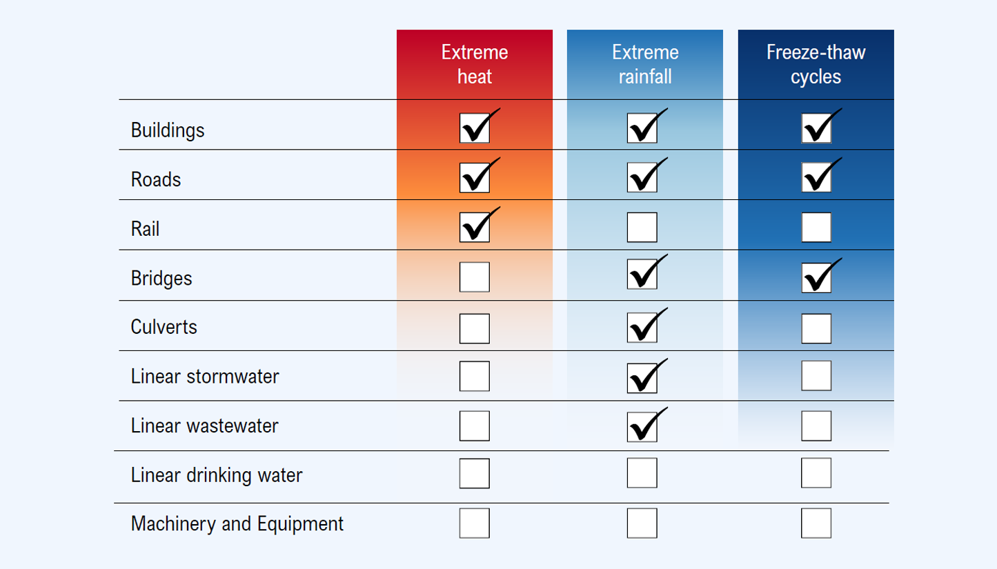
Source: WSP and FAO.
Figure 3‑2 shows which hazards WSP deemed most relevant to assess for each asset-type. High temperatures were expected to impact buildings, roads and rail infrastructure more significantly than other major asset classes. For example, underground linear drinking water and wastewater pipes are unlikely to be impacted by extreme heat. It was determined that extreme rainfall could have significant impacts on most asset classes. For freeze-thaw cycles, the most important impacts could occur on roads, but WSP determined that certain building and bridge components were also worth examining. It was determined that linear drinking water pipes and machinery and equipment assets were not expected to be significantly impacted by these three hazards and were excluded from the CIPI project.[89]
After the exclusion of drinking water and machinery and equipment assets, the scope of public infrastructure included in the CIPI project encompasses $193.5 billion of provincial infrastructure and $415.3 billion of municipal infrastructure. This represents 86.5 per cent of infrastructure assets examined in the FAO’s provincial and municipal reports. The omission of an interaction does not necessarily mean that these climate hazards will have no impact on the asset class, but rather that WSP indicated the impacts are less likely to be important.
Figure 3-3 Scope of provincial and municipal infrastructure by asset class in CIPI
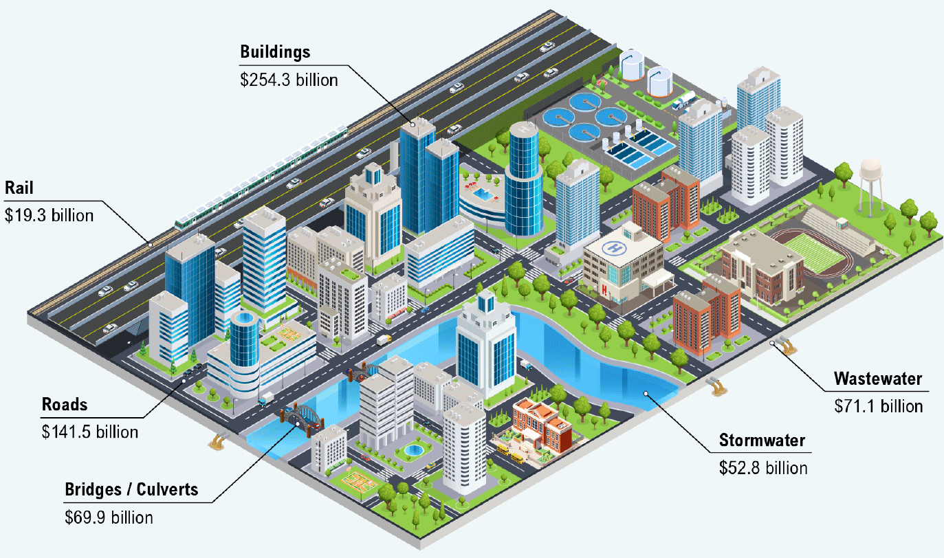
Source: FAO.
The FAO’s analysis is based on the current suite of public infrastructure assets. It does not include any assets either currently under construction, planned for future construction or necessary to meet future infrastructure demand. The analysis does not incorporate any functionality improvements to existing public infrastructure in the future. While these costs will be significant, estimating this spending and the associated climate-related costs are beyond the scope of the project.
The Long-term Costs of Maintaining Public Infrastructure
Infrastructure assets require ongoing capital and operating spending. Capital spending for existing infrastructure includes money spent on repairing assets through either rehabilitation[90] or renewal,[91] and occurs less frequently than operating costs, which take place annually and include operations and maintenance (O&M) expenses. Both costs are necessary to maintain infrastructure in a state of good repair, helping to ensure assets are delivering their intended services in a condition that is considered acceptable from both an engineering and a cost-management perspective.
To calculate these costs, the FAO used an infrastructure deterioration model, based on techniques developed by the Ontario Ministry of Infrastructure (MOI), in combination with provincial and municipal infrastructure data[92] to forecast the capital and operating expenses necessary to maintain assets in a state of good repair to 2100 in the absence of climate change considerations.[93]
The model determines these capital and operating expenses based on the individual characteristics of each particular asset. A new asset in very good condition requires less capital spending over the coming decades compared to an older asset in a poor state of repair. Similarly, one asset-type may have higher performance standards than another. Operating expenses could also vary based on asset-type.
Unlike the FAO’s previous reports, which assessed the state of repair of provincial and municipal infrastructure,[94] the third phase of the CIPI project begins by projecting the costs required to bring and maintain public infrastructure into a state of good repair over the long term in the absence of climate change considerations. This scenario forms the base case against which scenarios that include the impact of climate hazards are compared. In this way, the costs associated with climate change are distinguished from the costs associated with addressing the current and future infrastructure backlog.
For a detailed description of the infrastructure deterioration model, see the Appendix.
Climate Cost Elasticities
This section defines the concepts used to enhance the infrastructure deterioration model to incorporate climate change impacts. The section also briefly outlines how WSP developed the required model relationships referred to as “climate cost elasticities” for climate change damage costs and for the costs of climate change adaptation.
Defining Climate Change Costs in the Infrastructure Deterioration Model
Damage Costs
Damage costs are defined as the change in long-term infrastructure costs (relative to the base case) in the absence of any adaptation measures. These costs could be related to additional or more frequent rehabilitations and faster renewals, as well as changes to operations and maintenance expenses due to extreme events or accelerated weathering.
WSP developed two types of relationships between changes in climate variables and infrastructure damage costs. These costs would manifest in the absence of any adaptation actions.
- A change in useful service life (USL) due to a change in climate variable. Climate change will alter the historical deterioration patterns of infrastructure. Assets may deteriorate more rapidly (or more slowly in some cases) due to long term changes in key climate variables. In the infrastructure deterioration model, accelerated asset deterioration results in more frequent or additional rehabilitation costs, and in accelerated asset renewals (assets with shorter USLs need to be replaced sooner in the absence of rehabilitation).
- A change to operations and maintenance (O&M) expenses due to a change in climate variable. The cost of O&M may also be impacted by changing climate variables in the absence of adaptation measures. For example, more frequent inspections may be required, raising the annual cost of operations.
Adaptation Costs
Adapting public infrastructure to specific climate hazards could take many forms. In some cases, it might involve updating infrastructure design parameters to a higher standard.[95] In others, it might mean upgrading certain asset components to accommodate changing climatic conditions. Adaptation could also mean that infrastructure is redesigned or replaced with other options, such as the use of green infrastructure including planting trees, enhancing wetlands or installing green roofs instead of relying on stormwater pipes or ditches to accommodate higher rainfall intensities.
In this study, “adaptation costs” are defined as the cost of actions that would address the impacts of select climate hazards to ensure that assets perform to the same standards for which they were initially designed (e.g., stormwater pipes that would not overflow in more extreme rainfall events), and to prevent accelerated asset deterioration and additional O&M expenses despite changed climate variables.
WSP developed two types of relationships between changes in climate variables and infrastructure adaptation costs.
- The cost of retrofits to adapt to a change in climate variable. One adaptation option for asset managers is to retrofit an asset before the end of its service life. “Retrofit” in this project means replacing components of an asset with ones that are adapted to changed climate variables. The nature of these retrofits depends on an asset’s specific circumstances. For example, retrofitting include waterproofing a building’s foundation or shoring up road embankments to prevent accelerated erosion.[96]
- A change in the cost of asset renewal to adapt to a change in climate variable. Climate change adaptation can also occur at the end of an asset’s service life if it is replaced with one that is designed to withstand the changes in climate variables. Adaptations at renewal can only occur when an asset is fully replaced, while adaptation as a retrofit can occur at any point during the asset’s life.
Assumptions and rationales for damage and adaptation costs by asset class, component and climate hazard are detailed in the WSP report.
Estimating climate cost elasticities
WSP estimated a climate cost elasticity for each of the four types of relationships between changing climate variables and infrastructure costs as defined above. In general, an elasticity is a measure of one variable’s sensitivity to a change in another variable. In this case, the climate cost elasticity indicates the change in an aspect of infrastructure costs relative to a change in a specific climate variable.
For each climate hazard relevant for each asset class, WSP engineers consulted with their subject-matter experts (SMEs) and selected the most appropriate climate variable to proxy the hazard in question for each asset class and/or asset component. For instance, rail infrastructure is most impacted by extreme high temperatures. For rail track alignments the number of days with temperatures above 30°C was determined to be the most relevant climate indicator for extreme heat, while for rail-associated structures (e.g., noise walls) the mean July daily maximum temperature was the most relevant indicator.[97]
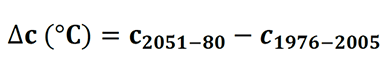
To estimate the required climate cost elasticities, WSP first calculated the change in the selected climate change indicators (represented as ∆c) under the RCP8.5 90th percentile scenario for three representative regions in Ontario (North, Centre and South). These estimates were used to benchmark the upper end of the possible range of values for consideration by WSP’s SMEs. For non-temperature-based indicators, this is calculated as a per cent change by late century (the average from 2051-2080) relative to the 1976-2005 baseline:

For temperature-based indicators measured in °C, this variable this is calculated as a level change:
Once estimated, WSP surveyed relevant SMEs, asking them to estimate the impact of these climate indicators on the various types of infrastructure costs. The survey questions appear in Table 3‑1.
| Type of cost | Question asked to SMEs | Output |
|---|---|---|
| Rehabilitation costs | By 2051-80 following high-range RCP8.5, what would be the variation of service life under the influence of the evolution of each climate hazard for each asset and component? | Estimation of the reduction of useful service life (per cent) for an entire asset and a share percentage for each asset component directly linked to the corresponding climate variable |
| O&M costs | What would it cost annually, as a share of the current replacement value, to operate and maintain the expected deterioration rate under climate conditions of 2051-80 following high-range RCP8.5? | Estimation of future O&M costs (as per cent of CRV) for an entire asset and a share percentage of each asset component directly linked to the corresponding climate variable. |
| Renewal costs | Imagine you are designing a brand-new climate resilient building that has the same expected functionality of the 1976-2005 period, but for climate conditions of 2051-80 under the high-range RCP8.5 scenario. What would be the cost as a share of the current CRV? | Estimation of renewal costs (as a per cent of CRV) for an entire asset and a share percentage for each asset component. |
| Retrofit costs | What would it cost to retrofit, as a share of current replacement value, to make the building resilient to climate change given the climate projections of a high-range RCP8.5? | Estimation of retrofit costs (as a per cent of CRV) for an entire asset and a share percentage for each asset component directly linked to the climate variable. |
WSP aggregated the survey results into a probability distribution with optimistic, pessimistic and most-likely values. The SMEs’ answers to these questions reflect their engineering knowledge of federal and provincial building codes, their understanding of the literature on climate-infrastructure interactions, the broad characteristics and nature of the assets in scope, and the average climate vulnerability of these assets. The cost estimates generated by the SMEs can be represented as ∆p. This value reflects the change in infrastructure cost given the change in climate (∆c).
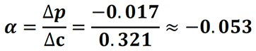
The ratio between ∆p and ∆c was used to calculate the climate cost elasticity expressed as the sensitivity of an infrastructure cost (in per cent) per variation in climate variable, represented by α:
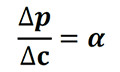
In general, a climate cost elasticity of zero (α = 0) implies that the climate change indicator has no impact on the infrastructure cost to which that elasticity is applied. For climate cost elasticities applied directly to infrastructure costs (including O&M expenses, retrofit and renewal costs), a positive value (α > 0) indicates that the respective infrastructure cost will increase as the climate indicator increases. A negative value (α < 0) indicates a cost reduction. For climate cost elasticities applied to USLs, a negative value indicates that the USL will decline as the climate indicator increases, and vice versa.
For example, the 15-minute rainfall intensity of a 10-year storm event is projected to increase by 32.1 per cent in Ontario by late century when compared to the historical baseline under the 90th percentile projections of RCP8.5. SMEs consulted by WSP determined that this change in rainfall intensity could reduce the USL of the average public building in Ontario by 1.7 per cent by 2051-2080 due to the negative impacts on building envelopes.[98] This corresponds to an elasticity of -0.053 for building envelopes, which indicates that for every 1.0 per cent increase in the 15-minute rainfall intensity of a 10-year event, the USL of the average public building in Ontario is expected to decline by 0.053 per cent. A shorter USL due to changes in extreme rainfall will raise infrastructure costs by hastening the need for rehabilitations and asset renewals.
In some cases, WSP engineers established climate cost elasticities between climate variables and different asset-types within an asset class. For example, separate elasticities for extreme rainfall cost impacts were estimated for pipes and ditches in the stormwater asset class, as extreme rainfall will impact these asset-types differently. In other cases, elasticities were estimated for individual components of assets. For example, climate cost elasticities were produced for six separate building components and the impacts of each were weighted together based on the average component share of the building’s current replacement value.[99]
Once estimated, the FAO integrated the climate cost elasticities (α) into the FAO’s infrastructure deterioration model and coupled them with the regional climate projections produced by Canadian Centre for Climate Services to estimate infrastructure cost impacts in different RCP scenarios (see Appendix A-1 for technical details).
Climate cost elasticities are assumed to be constant over time, implying a linear relationship between the changing climate indicator and the projected cost. This relationship is intuitive for chronic climate hazards, including extreme heat, freeze-thaw cycles and certain aspects of extreme rainfall (e.g., average annual precipitation or the maximum 5-day rainfall amount). However, there are other aspects of the rainfall hazard that include extreme events where observed financial effects are often distributed unevenly over time (e.g., the 100-year rain event). The FAO’s approach captures the impact of extreme rainfall events but assumes that they average out across large asset classes and regions over time.
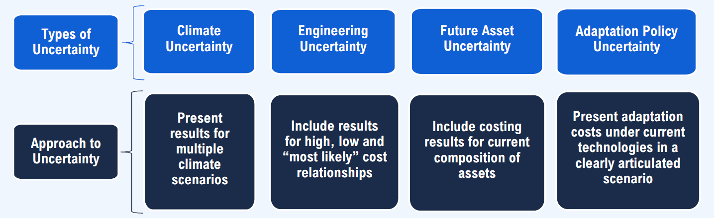
Presenting Costing Results and Accounting for Uncertainty
In presenting climate change damage cost and adaptation cost results over long periods of time, there are numerous uncertainties that must be acknowledged.
Damage Costs
Presenting costing results for a damage cost scenario can inform the extent to which asset owners could incur additional costs in the absence of adaptation actions. A damage cost scenario could be estimated for a “typical asset,” across an entire asset class, or for the entire portfolio of public assets under study.
For the damage cost results at the asset class level, the most important areas of uncertainty include climate uncertainty, engineering uncertainty, and asset composition uncertainty.
Climate Uncertainty
Since the future path of emissions and climate change is unknown, the FAO will provide damage cost results for RCP8.5 (the high emissions scenario) as well as for the RCP4.5 scenario (considered a “medium” emissions scenario) in the sector costing reports. The FAO may also present results for RCP2.6 as background information.
An additional climate uncertainty arises within each RCP scenario, as there are 24 different global models, each with its own results for how sensitive the earth’s climate will be to given levels of greenhouse gas concentrations. The sector costing reports will primarily present results for the median projection of each selected RCP, but will also present the range of possible outcomes by including results for the 10th and 90th percentile climate model simulations within each RCP scenario as uncertainty ranges.
Lastly, the latest IPCC report states that “Low-likelihood outcomes, such as ice sheet collapse, abrupt ocean circulation changes, some compound extreme events and warming substantially larger than the assessed very likely range of future warming cannot be ruled out…”[100] While the FAO’s methodology is intended to estimate the range of costs to public infrastructure in the most likely climate scenarios, it is not designed to account for these and other low-likelihood outcomes.
The IPCC points out that as global warming increases, extreme events that were infrequent in the past will become more frequent, and “…there will be a higher likelihood that events with increased intensities, durations and/or spatial extents unprecedented in the observational record will occur.”[101] As such, this issue is most prevalent for RCP8.5 and to a lesser extent for RCP4.5.
Engineering Uncertainty
WSP engineers were asked to develop a typical relationship between a given change in climate variable and infrastructure costs at the asset class level in Ontario. Within an asset class (e.g., “buildings”), there are variations that can add uncertainty to the engineering climate elasticities: assets built using different designs and according to different versions of the design code, assets that use different building materials in their construction, and assets that have varying degrees of vulnerability to changing climate variables. To account for these uncertainties, WSP estimated high, low and most likely cost relationships. The FAO costing reports will focus on the “most likely” relationships but will make available simulations based on the high and low estimates as background information.
In addition, public assets are in various states of repair. To control for the costs associated with bringing assets into a state of good repair, the FAO base case and climate scenario simulations assume that all assets are brought into a state of good repair at their earliest opportunity. In this way, climate change damage costs are expressed as a change in costs relative to the current state of good repair.
Future Asset Composition Uncertainty
Over the next three decades, Ontario’s population is projected to grow by between 20 per cent in a low scenario and 53 per cent in a high scenario.[102] Accommodating this population growth would require more public buildings like schools and hospitals, water systems, and transportation infrastructure. The FAO’s upcoming sector costing reports will focus on the current suite of public infrastructure assets, and will not include assets either currently under construction, planned for future construction or necessary to meet future infrastructure demand.
While this exclusion limits the scope of potential future climate change damage costs, it was not possible to reliably account for the uncertainty associated with future population growth, building technologies, and public infrastructure composition and demand in the sector reports. Future research could assess this issue.
Adaptation Costs
Damage costs scenarios are useful projections to gauge the costs of inaction on climate change adaptation. However, all levels of government, the private sector and many other institutions are working on various adaptation solutions. For example, the Ontario Ministry of Transportation assessed the resilience of highway drainage infrastructure under different climate change scenarios and identified possible adaptation measures.[103]
A wide range of adaptation options is currently available to asset managers, and options differ depending on the context, climate hazard and asset in question. Building codes will be updated, government policies will change, technology will evolve, and the actions of provincial and municipal asset owners will be influenced by their budgets. In considering adaptation actions, asset managers would likely consider an asset’s remaining useful life, the cost of adaptation, the importance of the asset’s services, the extent to which an asset’s services are compromised, and the condition of the asset, among other things. These considerations raise further uncertainties in estimating the costs of climate change in terms of adaptation costs.
Furthermore, adaptation decisions do not only depend on the asset itself. As public infrastructure provides vital services, including transportation, health and flood protection, any service interruption can have significant social and economic consequences. For this reason, and due to the significant additional uncertainties associated with what a broad adaptation strategy would look like, the CIPI project will not attempt a cost-benefit analysis that compares climate change damage and adaptation costs to society. To do so would require a much broader frame of analysis that includes, among other things, the costs of public infrastructure failure to society and the economy. As CIPI’s scope focuses on the financial impact to asset managers themselves, the project will instead present a range of possible adaptation costs to public infrastructure owners.
Strengths and Limitations of the FAO’s Approach
The FAO’s methodology has numerous strengths as well as some key caveats and limitations, outlined below.
Strengths
The FAO’s approach allows significant flexibility in evaluating the impact of climate change costs to infrastructure. This approach provides the ability to:
- model cost outcomes in different emissions scenarios;
- cost average climate impacts over the forecast horizon to capture long-term climate trends; and
- isolate the cost impact of specific climate hazards or cost types, such as climate impacts to O&M, rehabilitation or renewal costs.
As the model uses granular data on public assets including their age, condition, value and location, this can be coupled with downscaled regional climate projections to account for expected geographic variability of climate change in Ontario. In addition, the long-term costs in the base case and climate scenarios each incorporate the age structure of public infrastructure, and account for when public assets require investment over the coming decades and how climate hazards can impact this timing.
Limitations
The FAO’s approach also has some limitations.
- Climate cost elasticities were calculated for an average asset in Ontario, such as a typical building or a typical road segment. While the results are reasonable on an asset class basis, they may not be applicable for specific assets. Similarly, one climate cost elasticity is used for each asset type regardless of an asset’s condition or age. Assets in poorer condition or built to older design standards would be impacted differently by changing climate hazards than assets in better condition or built more recently. Further research could refine the climate cost elasticities along these lines.
- Climate cost elasticities were estimated at the provincial level and used in combination with regional climate projections. As such, regional results do not account for any potential regional engineering differences, either in infrastructure design or use of building materials.
- The FAO’s approach treats the impact of each climate hazard independently and does not account for the significant interdependencies between public infrastructure. Extreme weather events have often caused cascading infrastructure failures, such as storms that knock out power to basement sump pumps, leading to significant damage from basement flooding. In addition, multiple simultaneous hazards are not necessarily additive. The inability to adequately model these interdependencies is one reason the FAO’s damage costs should be considered lower-bound estimates.
- The project examines certain climate change impacts to infrastructure levels of service, for example, the installation of air conditioning in buildings to regulate temperatures, or the replacement of stormwater pipes whose capacity needs to be upgraded. Infrastructure deterioration models do not capture these types of impacts to service levels, and the assumptions required to include them are a source of additional uncertainty.
- Greenhouse gas mitigation is becoming increasingly integrated into infrastructure design management decisions, which can affect the cost of future construction and rehabilitation. Mitigation considerations were not included in this study and are a possible area of future research.
The FAO’s Results Should Be Seen as Lower-Bound Cost Impacts
In addition to excluding the impact of infrastructure interdependencies, there are other reasons why the FAO’s costing results should be viewed as lower-bound estimates.
- The scope of the project is limited to a subset of existing publicly owned provincial and municipal assets. Not assessed are the impacts of the changing climate to provincial and municipal machinery and equipment, federal and private infrastructure, or any new assets that could be built over the coming decades.
- This analysis assumes that all assets are kept in a state of good repair and that whatever capital or operating spending is needed is available and spent by the Province and Ontario’s municipalities. However, the FAO has estimated that significant infrastructure backlogs exist at both the provincial and municipal level. In the future, budget constraints may limit the ability of governments to address these backlogs, and assets in poorer condition are often more vulnerable to climate hazards.
- This analysis examines only a subset of the suite of relevant climate hazards to public infrastructure. While the FAO chose to focus on hazards where projections had a higher degree of scientific confidence, numerous potentially significant climate hazards such as wildfires and fluvial flooding were not included (see Chapter 2).
4 | Appendix
Infrastructure Deterioration Model
The infrastructure deterioration model used in this project is largely based on a modelling framework provided by the Ontario Ministry of Infrastructure and further developed by the FAO. The model evaluates infrastructure data through a series of simplified asset management decisions. While the model replicates decisions made by asset managers within this simple framework, it was designed principally as a financial model to estimate the costs of infrastructure and is not intended to replicate or predict specific interventions that asset managers make.
The model’s financial estimates are sensitive to the data and methodology used in this report. For example, asset managers may have different views on what is considered a “state of good repair” for a particular asset class. This makes assumptions necessary while recognizing that the definitions are subject to debate.[104]
Modelling Infrastructure Deterioration in the Absence of Climate Change
To model infrastructure deterioration and its associated costs in the absence of climate change, assets are plotted on standardized asset-type-specific deterioration curves. Most of these curves were developed by MOI and capital portfolio ministries and describe how asset conditions typically evolve over time.
Figure 4-1 Infrastructure deterioration modelling framework
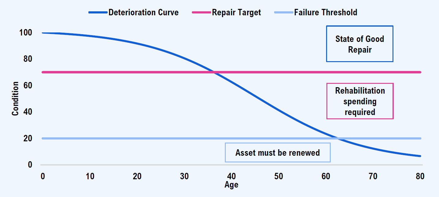
Source: FAO.
Accessible version
The figure shows a stylized deterioration curve.
The dark blue curve in Figure 4‑1 represents a stylized deterioration curve. An asset’s deterioration curve can also be described by the following equation:
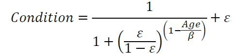
Where β and ε are asset-class-specific curve parameters[105] (see Table 4‑1) that determine the shape of each condition curve.
Assets deteriorate as they age and move down their respective deterioration curves and are evaluated against performance standards. These performance standards were largely provided to the FAO by MOI, except for water infrastructure assets (potable, storm and waste) which the FAO developed in consultation with WSP engineers. These performance standards determine what, if any, type of capital spending is required and include:
- Repair targets are the condition which, at or above, an asset does not require any current capital spending and is considered acceptable from both an engineering quality assessment and cost management perspective. Assets with conditions at or above the repair target are considered to be in a state of good repair.
- Failure thresholds are defined as the condition at which assets are beyond rehabilitation and should be replaced.
- Design Service Life (DSL) is defined as the number of years for which an asset is designed to remain in operation. Assets typically remain in use for longer than their design life. The FAO assumes that all asset-types can remain in operation for twice its DSL if the asset is rehabilitated in a timely manner. The FAO defines twice an asset’s DSL as its Useful Service Life (USL).
Based on the asset’s condition and performance standards in Table 4 1, the model applies the logic outlined in Table 4-2 to determine if capital spending is required, and if so what type. Once the type of capital spending is determined, this spending is applied to the applicable assets. The repair is then reflected in the asset’s updated condition
The model also estimates operating costs by incorporating asset-class-specific operations and maintenance (O&M) cost schedules. These operating costs occur annually. O&M costs are based on the CRV of assets. The FAO estimates O&M expenses based on the following equation:
where O&M share by asset class is calculated as the typical O&M spending relative to the asset’s CRV.
The performance standards for each asset-type used in the model are described in Table 4-1.
Asset managers must weigh the cost of repairs against a host of other considerations, all in the context of budget constraints. However, the model does not incorporate budget constraints and assumes all necessary capital and O&M spending is performed in the year required. This means that if an asset requires rehabilitation today, it will be performed and the asset will be brought into a state of good repair, either through rehabilitation or renewal.
Incorporating the Impact of Climate Hazards into the Model
To incorporate the impacts of select climate hazards into the modelling framework, several adjustments are made to the process described above. This includes adjusting the asset’s O&M share and USL, and adding adaptation as an option for capital spending decisions, either through retrofits or renewals.
These adjustments are made based on the climate hazard’s impact, determined by multiplying WSP’s climate cost elasticities by the percentage change (or level change for temperature-based indicators) of the relevant climate indicator. For damage costs, which include O&M expenses and a reduction in USL, the change in the climate hazard indicator from its base value is updated each decade to reflect the evolving climate. For adaptation costs, the change in the climate hazard indicator from its base value is calculated on the 2080 decadal average of the indicator. This is done so assets are adapted to future expected climate hazards, and not just for the current climate.
Once these adjustments are incorporated into the model, the model works in much the same way as it does in the base case scenario in the absence of climate change. Assets deteriorate and are assessed relative to performance standards. Assets are either left to deteriorate or repaired through either rehabilitation or renewal, while O&M expenses are incurred annually.
The following sections describe how each cost adjustment is made in the model. The adjustments presented in this section assume that all three climate hazards were assessed. This was the case for buildings, but for other asset-types, only one or two hazards were assessed.
Climate Hazard Impact on O&M Expenses
The impact of changes in select climate hazards on an asset’s O&M costs are based on the formula described below:
![〖O&M〗_CC=CRV× [O&M Share + α_(O&M,XR)×〖∆C〗_XR+α_(O&M,XH)×〖∆C〗_XH+α_(O&M,FTC)×〖∆C〗_FTC ]](/wp-content/uploads/report/EC1908-Climate-Change-and-Public-Infrastructure/images-en/formula-7.png)
where
- \(\alpha_{O \& M,XR}\) is the climate cost elasticity of extreme rainfall on O&M
- \(\Delta C_{XR}\) is the change[106] in the extreme rainfall indicator relative to the base period (1976-2005)
- \(\alpha_{O \& M,XH}\) is the climate cost elasticity of extreme heat on O&M
- \(\Delta C_{XH}\) is the change in the extreme heat indicator relative to the base period
- \(\alpha_{O \& M,FTC}\) is the climate cost elasticity of Freeze-Thaw Cycles on O&M
- \(\Delta C_{FTC}\) is the change in the freeze-thaw cycle indicator relative to the base period
However, if the asset has been adapted, O&M expenses revert to the original equation described above in the absence of climate change.
Climate Hazard Impact on Useful Service Life
The impact of changes in select climate hazards on an asset’s USL costs are based on the formula described below.
![〖USL〗_cc=USL× [1+ (α_(USL,XR)×〖∆C〗_XR+α_(USL,XH)×〖∆C〗_XH+α_(USL,FTC)×〖∆C〗_FTC )]](/wp-content/uploads/report/EC1908-Climate-Change-and-Public-Infrastructure/images-en/formula-9.png)
where
- \(\alpha_{USL,XR}\) is the climate cost elasticity of extreme rainfall on USL
- \(\Delta C_{XR}\) is the change in extreme rainfall indicator relative to the base period
- \(\alpha_{USL,XH}\) is the climate cost elasticity of extreme heat on USL
- \(\Delta C_{XH}\) is the change in extreme heat indicator relative to the base period
- \(\alpha_{USL,FTC}\) is the climate cost elasticity of Freeze-Thaw Cycles on USL
- \(\Delta C_{FTC}\) is the change in freeze-thaw cycle indicator relative to the base period
This updated climate hazard impacted USL (\(USL_{cc}\)) is then converted into a reduction in DSL by the following formula
The “climate adjusted design life” (\(DSL_{cc}\)) is then input into the formula below (which is a rearrangement of the original condition formula to solve for value of β).
![β_CC=〖DSL〗_cc/[1-log[1/(1-(1-Failure Threshold)-ε)]/log[ε/(1-ε)] ]](/wp-content/uploads/report/EC1908-Climate-Change-and-Public-Infrastructure/images-en/formula-11.png)
The “climate adjusted” β \(\beta_{cc}\) determines the asset’s new rate of deterioration after incorporating the impact of climate hazards on the asset’s USL. Figure 4‑2 shows a stylized representation of how a deterioration curve could vary after incorporating climate hazards, which typically (but not always) results in a decrease in the asset’s USL.
This updated rate of deterioration is used within the framework described in Table 4‑2 to calculate the asset’s required capital spending over time. This more rapid deterioration means the asset will fall out of a state of good repair sooner, requiring earlier and more frequent rehabilitation. In addition, the asset reaches its failure threshold sooner, resulting in an earlier renewal. This new deterioration rate is applied until an asset is adapted, at which point the deterioration curve reverts to its original shape (see renewal and retrofit adaptation below).
Figure 4-2 Incorporating climate hazards changes asset deterioration rate and USL
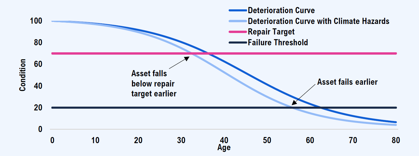
Source: FAO.
Accessible version
The figure shows a stylized deterioration curve with climate hazards.
Climate Hazard Impact on the Cost of Renewal Adaptations
Renewals are an adaptation option for buildings that occur at the end of their useful lives. Renewal is a one-time cost that is calculated based on the following formula.
![〖Renewal〗_cc=CRV× [1×(α_(RNW,XR)×〖∆C〗_XR+α_(RNW,XH)×〖∆C〗_XH+α_(RNW,FTC)×〖∆C〗_FTC )]](/wp-content/uploads/report/EC1908-Climate-Change-and-Public-Infrastructure/images-en/formula-12.png)
where
- \(\alpha_{RNW,XR}\) is the climate cost elasticity of extreme rainfall on renewal adaptation
- \(\Delta C_{XR}\) is the change in extreme rainfall indicator relative to the base period
- \(\alpha_{RNW,XH}\) is the climate cost elasticity of extreme heat on renewal adaptation
- \(\Delta C_{XH}\) is the change in extreme heat indicator relative to the base period
- \(\alpha_{RNW,FTC}\) is the climate cost elasticity of Freeze-Thaw Cycles on renewal adaptation
- \(\Delta C_{FTC}\) is the change in freeze-thaw cycle indicator relative to the base period
Once an asset is adapted via renewal, its CRV changes as well. The change in the asset’s CRV is equal to the cost of renewal adaptation given in the formula above. In practice, this means that O&M costs and capital expenditures will also reflect this change (i.e., if an asset’s adapted CRV is larger than its un-adapted CRV, O&M costs and future rehabilitation and renewal costs will also increase).
Once an asset is adapted via renewal, its deterioration curve and O&M expenses reflect this adaptation. If an asset is adapted to all climate change variables, its deterioration curve and O&M share revert to their original values. If an asset is adapted to one hazard but not to the other two hazards, its deterioration curve and O&M expenses reflect this selective adaptation.[107]
Climate Hazard Impact on the Cost of Retrofit Adaptations
Retrofits are an adaptation option for buildings that are not near the end of their useful lives. Within the model’s framework, retrofits occur at the same time as a rehabilitation.[108] For example, a new asset cannot be retrofitted until it has deteriorated below its state of good repair and is eligible for repair.
Retrofit expenses are one-time costs that are calculated using the following formula:

where
- \(\alpha_{RFT,XR}\) is the climate cost elasticity of extreme rainfall on retrofit adaptation
- \(\Delta C_{XR}\) is the change in extreme rainfall indicator relative to the base period
- \(\alpha_{RFT,XH}\) is the climate cost elasticity of extreme heat on retrofit adaptation
- \(\Delta C_{XH}\) is the change in extreme heat indicator relative to the base period
- \(\alpha_{RFT,FTC}\) is the climate cost elasticity of freeze-thaw cycles on retrofit adaptation
- \(\Delta C_{FTC}\) is the change in freeze-thaw cycle indicator relative to the base period
Once an asset is adapted through retrofit, its CRV changes as well. The change in the asset’s CRV is equal to the cost of renewal adaptation. This is given by the same formula used to calculated renewal adaptation costs described in the preceding sub-section. In practice, this means that O&M costs and capital expenditures will also reflect this change (e.g., if an asset’s adapted CRV is larger than its un-adapted CRV, O&M costs and future rehabilitation and renewal costs will also increase).
Once an asset is adapted via retrofits, its deterioration curve and O&M expenses reflect this adaptation. If an asset is adapted to all climate hazards, its deterioration curve and O&M reverts to its original curve in the absence of climate change. If an asset is adapted to one hazard but not to the other two hazards, its deterioration curve and O&M expenses reflect this selective adaptation.
| Sector | Asset Class | Asset Type | Repair Target |
Failure Threshold |
Beta | Epsilon | Design Service Life (Years) | Useful Service Life (Years) | O&M Share (% of CRV) |
|---|---|---|---|---|---|---|---|---|---|
| Transit | Buildings | 90 | 35 | 15.0 | 0.01 | 17 | 34 | 1.5% | |
| Engineering | 90 | 35 | 18.5 | 0.01 | 21 | 42 | 1.5% | ||
| Bridges and culverts | Engineering | New Bridges | 76 | 40 | 20.0 | 0.25 | 52 | 103 | 1.0% |
| Old Bridges, Deprecated | 76 | 45 | 20.0 | 0.20 | 36 | 72 | 1.0% | ||
| Roads | Engineering | Arterial Roads | 80 | 35 | 24.0 | 0.05 | 31 | 62 | 1.5% |
| Collector Roads | 75 | 40 | 19.0 | 0.15 | 31 | 62 | 1.5% | ||
| Freeways | 80 | 55 | 13.0 | 0.31 | 32 | 63 | 1.5% | ||
| Local Roads | 70 | 35 | 13.0 | 0.21 | 31 | 62 | 1.0% | ||
| Potable Water | Buildings | Potable Water Facilities | 70 | 15 | 45.0 | 0.02 | 67 | 134 | 1.5% |
| Storm Water | Buildings | Storm water facilities | 70 | 15 | 45.0 | 0.02 | 67 | 134 | 1.5% |
| Engineering | Small Pipes | 55 | 25 | 47.9 | 0.01 | 60 | 120 | 1.0% | |
| Medium Pipes | 55 | 25 | 51.0 | 0.01 | 64 | 128 | 1.0% | ||
| Large Pipes | 55 | 25 | 58.4 | 0.01 | 73 | 146 | 1.0% | ||
| Pipes of Unknown Diameter | 55 | 25 | 50.5 | 0.01 | 63 | 126 | 1.0% | ||
| Ditch | 55 | 25 | 41.5 | 0.01 | 52 | 104 | 1.0% | ||
| Culvert | 55 | 25 | 34.7 | 0.01 | 43 | 87 | 1.0% | ||
| Wastewater | Buildings | Wastewater Facilities | 70 | 15 | 45.0 | 0.02 | 67 | 134 | 1.5% |
| Engineering | Small Pipes | 60 | 30 | 56.2 | 0.01 | 67 | 134 | 1.0% | |
| Medium Pipes | 60 | 30 | 58.4 | 0.01 | 70 | 139 | 1.0% | ||
| Large Pipes | 60 | 30 | 61.7 | 0.01 | 74 | 147 | 1.0% | ||
| Pipes of Unknown Diameter | 60 | 30 | 52.8 | 0.01 | 63 | 126 | 1.0% | ||
| Sanitary Mains | 60 | 30 | 53.4 | 0.01 | 64 | 128 | 1.0% | ||
| Hospitals | Buildings | 79 | 20 | 30.0 | 0.01 | 39 | 78 | 1.5% | |
| Schools | Buildings | 80 | 20 | 30.0 | 0.01 | 39 | 78 | 1.4% | |
| Colleges | Buildings | 85 | 20 | 30.0 | 0.01 | 39 | 78 | 1.5% | |
| Other buildings and facilities | Buildings | Municipal Buildings and facilities | 80 | 20 | 35.0 | 0.02 | 49 | 97 | 1.5% |
| Government Administration & Ministry of Natural Resources and Forestry | 70 | 15 | 45.0 | 0.02 | 67 | 134 | 1.5% | ||
| Courthouses | 85 | 20 | 40.0 | 0.02 | 56 | 111 | 1.5% | ||
| Correctional facilities | 85 | 20 | 35.0 | 0.02 | 49 | 97 | 1.5% | ||
| Long-term care buildings | 79 | 20 | 30.0 | 0.01 | 39 | 79 | 1.5% | ||
| General Real Estate Portfolio | 80 | 20 | 35.0 | 0.02 | 49 | 98 | 1.5% | ||
| Engineering | Government Administration and Ministry of Natural Resources and Forestry | 72 | 20 | 39.0 | 0.01 | 51 | 102 | 1.5% |
| If the Asset’s… | Asset’s State of Repair | Capital Spending Required | Type of Capital Spending | Infrastructure Backlog |
|---|---|---|---|---|
|
In a State of Good Repair | No | N/A | Zero |
|
Not in a State of Good Repair | Yes | Rehabilitation | Amount necessary to bring asset’s condition to Repair Target[109] |
|
Not in a State of Good Repair | No | N/A | Zero. These assets will be allowed to deteriorate until Failure Threshold, at which point they will be renewed. |
|
Not in a State of Good Repair | Yes | Renewal | Amount equal to CRV |
5 | References
- Amec Foster Wheeler and Credit Valley Conservation, 2017, National Infrastructure and Buildings Working Group: Adaptation State of Play Report. Prepared for the Infrastructure and Buildings Working Group, part of Canada’s Climate Change Adaptation Platform.
- Bush, E. and Lemmen, D.S., editors, 2019, Canada’s Changing Climate Report, Government of Canada.
- Cannon, A.J., Jeong, D.I., Zhang, X., and Zwiers, F.W., 2020, Climate-Resilient Buildings and Core Public Infrastructure: An Assessment of the Impact of Climate Change on Climatic Design Data in Canada, Government of Canada.
- Council of Canadian Academies, 2019, Canada’s Top Climate Change Risks, The Expert Panel on Climate Change Risks and Adaptation Potential, Council of Canadian Academies.
- CSA Group, 2019, CSA Plus 4013:2019: Technical guide: Development, interpretation and use of rainfall intensity-duration-frequency (IDF) information: Guideline for Canadian water resources practitioners.
- Expert Panel on Climate Change Adaptation, 2009, Adapting to Climate Change in Ontario: Towards the Design and Implementation of a Strategy and Action Plan.
- Financial Accountability Office of Ontario, 2020, Provincial Infrastructure.
- Financial Accountability Office of Ontario, 2021, Municipal Infrastructure.
- Government of Ontario, 2011, Climate Ready: Ontario’s Adaptation Strategy and Action Plan.
- Government of Ontario, 2016, Climate Change Action Plan.
- Government of Ontario, 2018, Made-In Ontario Environment Plan.
- Government of Ontario. 2020, Protecting People and Property: Ontario’s Flooding Strategy.
- International Institute of Sustainable Development, 2021, Advancing the Climate Resilience of Canadian Infrastructure: A review of literature to inform the way forward.
- Intergovernmental Panel on Climate Change, 2013, Climate Change 2013: The Physical Science Basis: Annex II: Climate System Scenario Tables.
- Intergovernmental Panel on Climate Change, 2018, IPCC Special Report: Global Warming of 1.5°C: Summary for Policymakers.
- Intergovernmental Panel on Climate Change, 2021, Climate Change 2021: The Physical Science Basis: Summary for Policymakers.
- Office of the Auditor General of Canada, 2018, Perspectives on Climate Change in Canada: A Collaborative Report from Auditors General.
- Office of the Auditor General of Ontario, 2016, 2016 Annual Report of the Office of the Auditor General of Ontario.
- Office of the Auditor General of Ontario, 2019, An Overview of Environmental Issues in Ontario.
- Ontario Ministry of Transportation, 2015, The Resilience of Ontario Highway Drainage Infrastructure to Climate Change.
- Pacific Climate Impacts Consortium, 2021, PCIC Science Brief: Should the RCP 8.5 emissions scenario represent “business as usual?”.
- Task Force on Climate-related Financial Disclosures, 2017, Recommendations of the Task Force on Climate-related Financial Disclosures.
- Warren, F. and Lulham, N., editors, 2021, Canada in a Changing Climate: National Issues Report, Government of Canada.
- WSP, 2021, Costing climate change impacts and adaptation for provincial and municipal public infrastructure in Ontario, Deliverable #10 – Final Report, Toronto, Ontario. Report produced for Financial Accountability Office of Ontario.
| Areas of climate change risk | Agriculture and Food |
|---|---|
| Governance and Capacity | |
| Coastal Communities | |
| Human Health and Wellness | |
| Ecosystems | |
| Physical Infrastructure | |
| Fisheries | |
| Indigenous Ways of Life | |
| Forestry | |
| Northern Communities | |
| Geopolitical Dynamics | |
| Water | |
| Types of physical infrastructure affected by climate change | Residential |
| Electricity / Telecom | |
| Public | |
| Commercial | |
| Industrial | |
| Types of public infrastructure affected by climate change | Buildings |
| Transportation | |
| Water Infrastructure |
| Release Date | Report Title |
|---|---|
| Previously Released | Provincial Infrastructure |
| Municipal Infrastructure | |
| Fall 2021 | CIPI Project Backgrounder and Methodology |
| WSP Report | |
| Buildings and Facilities | |
| 2022 | Public Transportation Infrastructure |
| Public Water Infrastructure | |
| Summary Report |
| Year | Cumulative Carbon Dioxide emissions since 1850 (GtCO2) | Assessed global surface temperature relative to 1850-1900 (°C) | Human-caused warming (median estimate) (°C) |
|---|---|---|---|
| 1850 | 2.67 | -0.06 | -0.03 |
| 1900 | 194.48 | 0.12 | 0.06 |
| 1950 | 624.10 | 0.10 | 0.26 |
| 2000 | 1692.70 | 0.67 | 0.81 |
| 2019 | 2410.64 | 1.23 | 1.19 |
| Change in global mean temperature relative to pre-industrial period (°C) | Historical | RCP2.6 | RCP4.5 | RCP8.5 | |
|---|---|---|---|---|---|
| Historical | Pre-industrial period* | 0.0 | |||
| 1976-2005 | 0.6 | ||||
| Projection | 2010 | 1.0 | 1.0 (0.8 to 1.2) |
1.0 (0.8 to 1.2) |
1.0 (0.8 to 1.2) |
| 2020 | 1.2 | 1.2 (1.0 to 1.7) |
1.2 (1.0 to 1.4) |
1.3 (1.0 to 1.6) |
|
| 2030 | 1.4 (1.1 to 1.9) |
1.5 (1.2 to 1.8) |
1.6 (1.3 to 2.0) |
||
| 2040 | 1.5 (1.1 to 2.1) |
1.7 (1.3 to 2.2) |
1.9 (1.5 to 2.4) |
||
| 2050 | 1.6 (1.1 to 2.3) |
1.9 (1.5 to 2.6) |
2.3 (1.8 to 3.0) |
||
| 2060 | 1.5 (1.0 to 2.3) |
2.1 (1.5 to 2.8) |
2.8 (2.2 to 3.6) |
||
| 2070 | 1.5 (0.8 to 2.3) |
2.2 (1.6 to 2.9) |
3.2 (2.6 to 4.2) |
||
| 2080 | 1.6 (0.8 to 2.4) |
2.2 (1.6 to 3.2) |
3.7 (2.9 to 4.8) |
||
| 2090 | 1.6 (0.8 to 2.4) |
2.3 (1.7 to 3.2) |
4.2 (3.2 to 5.4) |
| Economic regions of Ontario |
|---|
| Hamilton–Niagara Peninsula |
| Kingston–Pembroke |
| Kitchener–Waterloo–Barrie |
| London |
| Muskoka–Kawarthas |
| Northeast A |
| Northeast B |
| Northeast C |
| Northwest A |
| Northwest B |
| Northwest C |
| Ottawa |
| Stratford–Bruce Peninsula |
| Toronto |
| Windsor–Sarnia |
| Year | Change in global mean temperature relative to 1976-2005 (°C) | Change in Ontario mean temperature relative to 1976-2005 (°C) |
|---|---|---|
| 1976-2005 | 0.0 | 0.0 |
| 2000 | 0.2 | 0.6 |
| 2010 | 0.5 (0.3 to 0.7) | 1.2 (0.8 to 1.4) |
| 2020 | 0.8 (0.5 to 1.1) | 1.7 (1.1 to 2.3) |
| 2030 | 1.0 (0.7 to 1.5) | 2.3 (1.5 to 2.9) |
| 2040 | 1.4 (1.0 to 1.9) | 3.0 (2.1 to 3.9) |
| 2050 | 1.8 (1.3 to 2.5) | 3.9 (2.8 to 4.9) |
| 2060 | 2.3 (1.6 to 3.1) | 4.7 (3.5 to 6.3) |
| 2070 | 2.7 (2.1 to 3.7) | 5.5 (4.2 to 7.3) |
| 2080 | 3.1 (2.4 to 4.3) | 6.3 (4.8 to 8.5) |
| 2090 | 3.7 (2.7 to 4.9) | 7.2 (5.4 to 9.9) |
| Climate hazards | Description | |
|---|---|---|
| Included (Based on potential impact on infrastructure and higher scientific confidence in climate projections) |
Extreme heat | Average and extreme temperature variables |
| Extreme rainfall | Total and extreme short-duration precipitation variables | |
| Freeze-thaw cycles | Daily maximum and minimum temperature and precipitation variables | |
| Excluded (Based on limited expected impact on infrastructure and/or lower scientific confidence in climate projections) Drought |
Ice storms | |
| Wildfires | ||
| Sea level rise | ||
| Permafrost melt | ||
| Windstorms |
| Ontario annual mean temperature (°C) | Historical | RCP2.6 | RCP4.5 | RCP8.5 | |
|---|---|---|---|---|---|
| Historical | 1950 | 0.2 | |||
| 1960 | 0.4 | ||||
| 1970 | -0.1 | ||||
| 1980 | 0.2 | ||||
| 1990 | 0.5 | ||||
| 2000 | 1.1 | ||||
| Projection | 2010 | 1.4 (0.4 to 2.0) |
1.4 (0.5 to 2.1) |
1.2 (0.5 to 2.4) |
|
| 2020 | 2.0 (1.1 to 2.9) |
1.2 (0.4 to 2.7) |
1.8 (0.6 to 2.8) |
||
| 2030 | 2.2 (1.2 to 3.0) |
1.9 (1.0 to 3.3) |
2.8 (1.7 to 3.7) |
||
| 2040 | 2.3 (1.4 to 3.6) |
2.9 (1.3 to 4.3) |
3.2 (1.2 to 4.0) |
||
| 2050 | 2.9 (1.9 to 3.6) |
3.2 (1.4 to 4.2) |
4.1 (2.7 to 5.1) |
||
| 2060 | 2.8 (1.4 to 4.6) |
3.3 (2.1 to 4.8) |
4.9 (3.1 to 6.9) |
||
| 2070 | 2.5 (0.8 to 3.9) |
3.7 (2.6 to 4.9) |
5.9 (4.4 to 7.4) |
||
| 2080 | 2.7 (1.9 to 4.2) |
3.9 (2.6 to 5.8) |
6.5 (4.8 to 8.7) |
||
| 2090 | 2.5 (1.2 to 4.0) |
4.4 (2.2 to 6.2) |
7.4 (5.0 to 9.3) |
||
| 2100 | 2.6 (1.6 to 4.0) |
3.6 (2.4 to 5.7) |
7.8 (6.0 to 10.4) |
| Economic region | Median projected change in annual mean temperatures from 1976-2005 to 2071-2100, RCP8.5 (°C) |
|---|---|
| Hamilton–Niagara Peninsula | 5.6 |
| Kingston–Pembroke | 5.7 |
| Kitchener–Waterloo–Barrie | 5.6 |
| London | 5.6 |
| Muskoka–Kawarthas | 5.6 |
| Northeast A | 5.9 |
| Northeast B | 6.1 |
| Northeast C | 6.2 |
| Northwest A | 6.2 |
| Northwest B | 6.2 |
| Northwest C | 6.7 |
| Ottawa | 5.7 |
| Stratford–Bruce Peninsula | 5.7 |
| Toronto | 5.6 |
| Windsor–Sarnia | 5.6 |
| Ontario total annual precipitation (mm) | Historical | RCP2.6 | RCP4.5 | RCP8.5 | |
|---|---|---|---|---|---|
| Historical | 1950 | 676 | |||
| 1960 | 659 | ||||
| 1970 | 653 | ||||
| 1980 | 667 | ||||
| 1990 | 708 | ||||
| 2000 | 689 | ||||
| Projection | 2010 | 716 (660 to 757) |
721 (648 to 756) |
719 (634 to 780) |
|
| 2020 | 716 (652 to 797) |
745 (669 to 783) |
699 (641 to 793) |
||
| 2030 | 708 (653 to 772) |
700 (630 to 773) |
708 (646 to 802) |
||
| 2040 | 719 (684 to 793) |
720 (657 to 800) |
745 (657 to 837) |
||
| 2050 | 736 (656 to 813) |
747 (662 to 821) |
759 (659 to 814) |
||
| 2060 | 708 (605 to 789) |
746 (634 to 803) |
746 (681 to 806) |
||
| 2070 | 757 (628 to 803) |
715 (656 to 819) |
796 (662 to 871) |
||
| 2080 | 729 (619 to 797) |
749 (639 to 840) |
769 (683 to 813) |
||
| 2090 | 749 (650 to 803) |
738 (660 to 814) |
810 (721 to 872) |
||
| 2100 | 736 (659 to 847) |
771 (671 to 829) |
806 (636 to 896) |
| Economic region | Median projected per cent change in total annual precipitation from 1976-2005 to 2071-2100, RCP8.5 (per cent) |
|---|---|
| Hamilton–Niagara Peninsula | 13.1 |
| Kingston–Pembroke | 14.1 |
| Kitchener–Waterloo–Barrie | 13.4 |
| London | 13.7 |
| Muskoka–Kawarthas | 13.8 |
| Northeast A | 14.2 |
| Northeast B | 16.3 |
| Northeast C | 15.6 |
| Northwest A | 14.0 |
| Northwest B | 11.3 |
| Northwest C | 15.3 |
| Ottawa | 13.4 |
| Stratford–Bruce Peninsula | 13.8 |
| Toronto | 13.7 |
| Windsor–Sarnia | 13.3 |
| Ontario annual number of freeze-thaw cycles | Historical | RCP2.6 | RCP4.5 | RCP8.5 | |
|---|---|---|---|---|---|
| Historical | 1950 | 80 | |||
| 1960 | 80 | ||||
| 1970 | 80 | ||||
| 1980 | 75 | ||||
| 1990 | 76 | ||||
| 2000 | 77 | ||||
| Projection | 2010 | 75 (67 to 88) |
71 (61 to 86) |
72 (60 to 86) |
|
| 2020 | 72 (63 to 84) |
73 (59 to 85) |
70 (58 to 88) |
||
| 2030 | 75 (61 to 85) |
70 (59 to 84) |
73 (59 to 82) |
||
| 2040 | 73 (62 to 91) |
69 (57 to 87) |
65 (56 to 89) |
||
| 2050 | 72 (59 to 84) |
71 (57 to 83) |
68 (56 to 83) |
||
| 2060 | 74 (60 to 86) |
69 (53 to 84) |
68 (52 to 83) |
||
| 2070 | 75 (62 to 88) |
67 (56 to 78) |
68 (53 to 85) |
||
| 2080 | 74 (56 to 88) |
66 (50 to 83) |
66 (56 to 82) |
||
| 2090 | 75 (56 to 85) |
69 (55 to 86) |
69 (53 to 85) |
||
| 2100 | 76 (60 to 89) |
67 (48 to 87) |
63 (48 to 81) |
| Economic region | Median projected per cent change in annual freeze-thaw cycles from 1976-2005 to 2071-2100, RCP 8.5 (per cent) |
|---|---|
| Hamilton–Niagara Peninsula | -36.4 |
| Kingston–Pembroke | -18.8 |
| Kitchener–Waterloo–Barrie | -23.6 |
| London | -34.2 |
| Muskoka–Kawarthas | -20.4 |
| Northeast A | -16.5 |
| Northeast B | -13.2 |
| Northeast C | -17.0 |
| Northwest A | -14.5 |
| Northwest B | -13.3 |
| Northwest C | -12.0 |
| Ottawa | -21.4 |
| Stratford–Bruce Peninsula | -28.1 |
| Toronto | -29.7 |
| Windsor–Sarnia | -38.1 |
| Winter rain intensity (mm/winter day) | Historical | RCP2.6 | RCP4.5 | RCP8.5 | |
|---|---|---|---|---|---|
| Historical | 1950 | 0.8 | |||
| 1960 | 0.8 | ||||
| 1970 | 0.8 | ||||
| 1980 | 0.7 | ||||
| 1990 | 0.8 | ||||
| 2000 | 0.8 | ||||
| Projection | 2010 | 0.8 (0.7 to 1.0) |
0.8 (0.6 to 0.9) |
0.8 (0.6 to 1.0) |
|
| 2020 | 0.8 (0.6 to 1.0) |
0.8 (0.7 to 1.0) |
0.7 (0.6 to 1.0) |
||
| 2030 | 0.8 (0.6 to 1.0) |
0.8 (0.7 to 1.0) |
0.8 (0.7 to 1.0) |
||
| 2040 | 0.9 (0.7 to 1.0) |
0.8 (0.6 to 1.0) |
0.8 (0.7 to 1.0) |
||
| 2050 | 0.9 (0.7 to 1.1) |
0.9 (0.6 to 1.0) |
0.9 (0.7 to 1.1) |
||
| 2060 | 0.8 (0.7 to 0.9) |
0.8 (0.6 to 1.1) |
0.9 (0.7 to 1.1) |
||
| 2070 | 0.8 (0.7 to 1.0) |
0.8 (0.6 to 1.0) |
0.9 (0.7 to 1.1) |
||
| 2080 | 0.8 (0.7 to 1.0) |
0.8 (0.6 to 1.0) |
0.9 (0.7 to 1.2) |
||
| 2090 | 0.8 (0.7 to 1.0) |
0.9 (0.6 to 1.0) |
1.0 (0.8 to 1.2) |
||
| 2100 | 0.9 (0.7 to 1.1) |
0.8 (0.7 to 1.0) |
1.0 (0.7 to 1.2) |
| Inputs | Climate Variable Projections |
|---|---|
| Provincial and Municipal Asset Inventories | |
| Climate Cost Elasticities (relationships between climate variables and infrastructure costs) |
|
| Model | Infrastructure Deterioration Model |
| Output | Financial impacts of selected climate hazards on public infrastructure |
| Public asset classes | Relevant climate hazards |
|---|---|
| Buildings | Extreme heat |
| Extreme rainfall | |
| Freeze-thaw cycles | |
| Roads | Extreme heat |
| Extreme rainfall | |
| Freeze-thaw cycles | |
| Rail | Extreme heat |
| Bridges | Extreme rainfall |
| Freeze-thaw cycles | |
| Culverts | Extreme rainfall |
| Linear stormwater | Extreme rainfall |
| Linear wastewater | Extreme rainfall |
| Linear drinking water | None |
| Machinery and Equipment | None |
| Asset class | Current replacement value ($ billions) |
|---|---|
| Buildings | 254.3 |
| Rail | 19.3 |
| Roads | 141.5 |
| Bridges / Culverts | 69.9 |
| Stormwater | 52.8 |
| Wastewater | 71.1 |
| Types of Uncertainty | Approach to Uncertainty |
|---|---|
| Climate Uncertainty | Present results for multiple climate scenarios |
| Engineering Uncertainty | Include results for high, low and “most likely” cost relationships |
| Future Asset Uncertainty | Include costing results for current composition of assets |
| Adaptation Policy Uncertainty | Present adaptation costs under current technologies in a clearly articulated scenario |
Footnotes
[1] Intergovernmental Panel on Climate Change, 2021.
[2] Bush, E. and Lemmen, D.S., editors, 2019, Section 8.4.2.3.
[3] Ibid, Table 4.2, Range is from the 25th percentile projection of RCP2.6 to the 75th percentile projection of RCP8.5.
[4] Council of Canadian Academies, 2019.
[5] Warren, F. and Lulham, N., editors, 2021, page 12.
[6] International Institute of Sustainable Development, 2021, page iv.
[7] Cannon, A.J., Jeong, D.I., Zhang, X., and Zwiers, F.W., 2020.
[8] Climate change adaptation plans and actions, Government of Canada. Government of Ontario, 2018.
[9] Office of the Auditor General of Canada, 2018.
[10] Canada’s Climate Change Adaptation Platform, Natural Resources Canada.
[11] Amec Foster Wheeler and Credit Valley Conservation, 2017.
[12] Climatic design data inform infrastructure design decisions and are contained in the National Building Code and other design codes.
[13] Cannon, A.J., Jeong, D.I., Zhang, X., and Zwiers, F.W., 2020.
[14] Climate-Resilient Buildings and Core Public Infrastructure Initiative, Government of Canada.
[15] Warren, F. and Lulham, N., editors, 2021.
[16] Canada’s National Adaptation Strategy, Government of Canada.
[17] Expert Panel on Climate Change Adaptation, 2009.
[18] Government of Ontario, 2011.
[19] Office of the Auditor General of Ontario, 2016.
[20] Government of Ontario, 2016.
[21] Infrastructure for Jobs and Prosperity Act, Government of Ontario, 2015.
[22] O. Reg. 588/17: Asset Management Planning for Municipal Infrastructure, Government of Ontario, 2017.
[23] Office of the Auditor General of Ontario, 2019.
[24] Government of Ontario, 2020.
[25] News Release: Ontario Launches First-Ever Climate Change Impact Assessment, Government of Ontario, 2020.
[26] For example, see Insurance Bureau of Canada and The Institute for Catastrophic Loss Reduction.
[27] See: The PIEVC protocol.
[28] Task Force on Climate-related Financial Disclosures, 2017.
[29] For example, see Under Water: The Costs of Climate Change for Canada’s Infrastructure, Canadian Institute for Climate Choices, 2021. Or: Investing in Canada’s future: The cost of climate adaptation, Federation of Canadian Municipalities, 2019.
[30] Financial Accountability Office of Ontario, 2020.
[31] Financial Accountability Office of Ontario, 2021.
[32] For example, if a culvert fails and a road washes out, the project would include the costs to governments of replacing the culvert and road, but would exclude the costs to surrounding homeowners or businesses of any basement flooding or road service disruption that might have occurred as a result.
[34] Bush, E. and Lemmen, D.S., editors, 2019, Chapter 2.
[35] Intergovernmental Panel on Climate Change, 2021, A.1.2.
[36] Ibid. Figure SPM.10.
[37] Ibid. A.1.
[38] Ibid. A.3.
[39] See: the IPCC’s Fifth Assessment Synthesis Report.
[40] In the long term, global temperatures are impacted by the difference between the incoming radiant energy from the sun and the outgoing radiation reflected out into space. If the incoming energy to Earth is greater than the outgoing energy, the planet will gradually warm. Higher concentrations of greenhouse gases in the atmosphere reduce outgoing heat from Earth, leading to a warmer climate. “Radiative forcing” is the term that describes the change in energy caused by natural or human made factors including greenhouse gas concentrations and is measured in watts per square metre (W/m2). For example, radiative forcing under the RCP8.5 scenario reaches roughly 8.5 W/m2 by 2100.
[41] Intergovernmental Panel on Climate Change, 2013, Table All.7.5. Ranges represent the 5th percentile to the 95th percentile projections of models used.
[42] Pacific Climate Impacts Consortium, 2021.
[43] Intergovernmental Panel on Climate Change, 2013, Table All.7.5. Ranges were adjusted to the pre-industrial base period.
[44] Intergovernmental Panel on Climate Change, 2018.
[45] By the end of the 21st century, global mean temperatures under RCP2.6 are projected to rise to 0.8-2.4°C above pre-industrial levels, with a median increase of 1.6°C. See Intergovernmental Panel on Climate Change, 2013, Table All.7.5. Ranges were adjusted to the pre-industrial base period.
[47] The CCCS extracted daily climate data from the BCCAQv2 dataset for individual climate model simulations. All data processing was carried out by the CCCS on a Linux compute cluster, primarily using the Python “xarray” and “xclim” processing packages within a Python 3.8 virtual environment.
[48] The Bias Correction/Constructed Analogues with Quantile mapping reordering Version 2 (BCCAQv2) dataset is an approximately 10 kilometre resolution nationwide ensemble of statistically downscaled climate model simulations of temperature and precipitation based on the multi-model Coupled Model Intercomparison Project 5. For more information on downscaling methods, see Pacific Climate Impacts Consortium, Climatedata.ca or Climate Data for a Resilient Canada.
[49] Bush, E. and Lemmen, D.S., editors, 2019.
[51] RCP6.0 projections are available from fewer models than the other scenarios. See Bush, E. and Lemmen, D.S., editors, 2019, page 131.
[52] See Technical documentation: Statistically downscaled climate scenarios, Government of Canada, and Climatedata.ca: About the BCCAQv2 time-series and maps.
[53] The IPCC’s sixth assessment (AR6) contains five scenarios of global socioeconomic change called Shared Socioeconomic Pathways (SSPs), which were lined up with the RCPs from AR5 in terms of average warming. This means that the scientific understanding of future climate change associated with RCPs is still relevant. In addition, the SSP global projections have yet to be regionally downscaled for Ontario. For these reasons, the CIPI project uses the RCP projections from the IPCC’s AR5 assessment.
[54] Pacific Climate Impacts Consortium, 2021.
[55] In addition, the 10th percentile projection for RCP4.5 represents a level of warming equivalent to median projections from RCP2.6.
[56] See Statistics Canada’s definition of economic regions.
[58] The Clausius-Clapeyron approach is described in CSA Group, 2019.
[59] Cannon, A.J., Jeong, D.I., Zhang, X., and Zwiers, F.W., 2020, Chapter 4.2.
[60] Approximately 0.6°C of anthropogenic warming has occurred from the pre-industrial era to the 1976-2005 average in both the global mean and Ontario average temperatures.
[61] Global mean temperature rose by around 1.1⁰C between 1950 and 2019. Intergovernmental Panel on Climate Change, 2021, Figure SPM.1.
[62] Bush, E. and Lemmen, D.S., editors, 2019, Chapter 2.
[63] Ibid, Chapter 4.
[64] Ibid, Chapter 5.
[65] Figures 2-2 and 2-4 use the same data for global mean temperatures. Temperature change in Figure 2-2 is expressed relative to 1850-1900 to discuss key global temperature thresholds. Temperature change in Figure 2-4 is relative to 1976-2005 to compare with CCCS data for Ontario.
[66] These figures approximately align with those found in Cannon, A.J., Jeong, D.I., Zhang, X., and Zwiers, F.W., 2020, Figure 2.4.
[67] Intergovernmental Panel on Climate Change, 2013, Table All.7.5. Ranges were adjusted to the pre-industrial base period.
[68] International Institute of Sustainable Development, 2021.
[69] Scientific confidence in climate projections differ by variable. In general, temperature projections have high scientific confidence due to a large body of evidence on the causes of observed changes and a strong understanding of the climate processes involved. Precipitation projections have medium scientific confidence due to inadequate observations for some historical variables and uncertainty associated with a weaker observed effect of global warming on precipitation. Other climate variables such as wind pressures and snow load have low scientific confidence due to a limited understanding of the climate processes involved. For more information, see Cannon, A.J., Jeong, D.I., Zhang, X., and Zwiers, F.W., 2020.
[70] Cannon, A.J., Jeong, D.I., Zhang, X., and Zwiers, F.W., 2020, Chapter 5.
[71] See Figures SPM.3 and SPM.5 in Intergovernmental Panel on Climate Change, 2021.
[72] Bush, E. and Lemmen, D.S., editors, 2019, page 239.
[73] To account for uncertainty in climate projections and in line with common practice in climate science, the median (50th percentile) projections for climate variables are presented, followed by ranges in parentheses. The ranges indicate the 10th and 90th percentile projections from the ensemble of 24 climate models used by the CCCS.
[74] Number of days in a year when the daily maximum temperature is above 30°C.
[75] Total degrees Celsius in a year when the daily mean temperature is above 18°C. An increase in cooling degree days means more air conditioning will be required.
[76] Cannon, A.J., Jeong, D.I., Zhang, X., and Zwiers, F.W., 2020, Section 1.2. Intergovernmental Panel on Climate Change, 2021, Figure SPM.3 and Section D.1.
[77] Bush, E. and Lemmen, D.S., editors, 2019, Table 4.4.
[78] Ibid, page 168.
[79] For IDF variables, the per cent changes for each RCP scenario are identical because the same mean temperature projection is used in the Clausius–Clapeyron relation to estimate the projections.
[80] Cannon, A.J., Jeong, D.I., Zhang, X., and Zwiers, F.W., 2020, Section 1.2. Intergovernmental Panel on Climate Change, 2021, Figure SPM.3 and Sections B.3 and C.2.
[81] Bush, E. and Lemmen, D.S., editors, 2019, page 308.
[82] “Rain” is defined as precipitation on days when the average temperature is above zero.
[83] “Winter” is defined as the period between the first and last frost day of the year. This definition is used because this period is shrinking due to climate change.
[84] Cannon, A.J., Jeong, D.I., Zhang, X., and Zwiers, F.W., 2020, Section 1.2.
[85] For a detailed description of the relationship between infrastructure and climate hazards developed by WSP and the full methodology underpinning their results, see WSP, 2021.
[86] Financial Accountability Office of Ontario, 2020.
[87] For more information on the current state of repair of provincial and municipal infrastructure, see Financial Accountability Office of Ontario, 2020, and Financial Accountability Office of Ontario, 2021.
[88] The CRV of provincially owned roads and highways has been revised with updated unit cost received from the Ontario Ministry of Transportation’s Parametric Estimating Guide 2016.
[89] WSP’s report contains the full engineering rationale for the selection of these hazard–asset class interactions.
[90] Rehabilitation is the repair of all or part of an asset, extending its life beyond that of the original asset, without adding to its capacity, functionality or performance. Rehabilitation is different from maintenance, which is the routine activities performed on an asset that maximize service life and minimize service disruptions. Assets are rehabilitated to a state of good repair (the repair target) and not to a new condition.
[91] Renewal is the replacement of an existing asset, resulting in a new or as-new asset with an equivalent capacity, functionality and performance as the original asset. Renewal is different from rehabilitation, as renewal rebuilds the entire asset.
[92] Asset data for provincial infrastructure were gathered from engineering-based asset-level assessments and high-level asset information provided by various ministries of the Ontario government. Asset data for municipal infrastructure were gathered from municipal asset datasets, asset management plans (AMPs), Canada’s Core Infrastructure Survey (CCPI) 2018, the Financial Information Return 2018, and the Ministry of Infrastructure Municipal Asset Inventory. For a description of provincial and municipal infrastructure data as well as data sources, see the appendices of Financial Accountability Office of Ontario, 2020, and Financial Accountability Office of Ontario, 2021.
[93] For a detailed description of the infrastructure deterioration model, see the Appendix.
[94] The reports also provided estimates of the level of outstanding capital spending necessary to bring assets into a state of good repair. This concept is referred to in the FAO’s provincial and municipal reports as the infrastructure backlog. For a more detailed discussion of the backlog and how it was calculated, see Financial Accountability Office of Ontario, 2020, and Financial Accountability Office of Ontario, 2021.
[95] Cannon, A.J., Jeong, D.I., Zhang, X., and Zwiers, F.W., 2020.
[98] WSP cited effects on sealants, increased water penetration in walls and interiors, and overloaded internal drainage systems, all of which contribute to leakage and failure. See WSP, 2021, for the full suite of engineering rationales that underpin the climate elasticities.
[100] Intergovernmental Panel on Climate Change, 2021, page 41.
[101] Ibid.
[102] See the Ontario Ministry of Finance’s population projections.
[103] Ontario Ministry of Transportation, 2015.
[104] The Province and Ontario’s municipalities manage a diverse portfolio of assets and may use different methodologies to determine the capital and operating spending costs of their assets.
[105] β determines the speed at which an asset deteriorates, while ε indicates an asset’s lowest allowable condition.
[106] Yearly climate indicators are smoothed into average values per decade to remove annual variation and capture only longer-term trends.
[107] For example, if an asset is adapted to extreme heat and extreme rainfall, but not to freeze-thaw cycles, the asset’s deterioration curve will no longer reflect the impact of extreme heat and extreme rainfall but will reflect the impact of freeze-thaw cycles. This same principle applies to O&M.
[108] While asset managers undertake retrofits whenever they decide is appropriate, retrofits and rehabilitation occurtogether to simplify possible decisions within the model.
[109] To estimate the cost of rehabilitation, the FAO assumes a direct relationship between an asset’s measured condition and its current replacement value. For example, if an asset’s condition index is 70 and its Repair Target is 85, rehabilitation costs are calculated by multiplying the asset’s CRV by the difference between the Repair Target and current condition, that is, CRV x [(85-70)/100]. For assets measured with a Facility Condition Index (FCI), this is true based on the definition and calculation of FCI. However, for assets measured using a Pavement Condition Index (PCI), Bridge Condition Index (BCI) or other technique this relationship is assumed. Asset managers may use different approaches to address the rehabilitation and renewal needs of their assets.